---
title: "Goodfellow Deep Learning — Deep Learning Book 6.3: Hidden Units and Activation Functions"
author: "Chao Ma"
date: "2025-09-29"
categories: ["Deep Learning", "Activation Functions", "Neural Networks"]
code-fold: true
code-summary: "Show code"
---
*This exploration of Deep Learning Chapter 6.3 reveals how activation functions shape the behavior of hidden units in neural networks - and why choosing the right one matters.*
📓 **For the complete implementation with additional exercises**, see the [notebook on GitHub](https://github.com/ickma2311/foundations/blob/main/deep_learning/chapter6/6.3/exercises.ipynb).
📚 **For theoretical background and summary**, see the [chapter summary](https://github.com/ickma2311/foundations/blob/main/deep_learning/chapter6/6.3/hidden_units_summary.md).
## Why Activation Functions Matter
Linear transformations alone can only represent linear relationships. No matter how many layers you stack, $W_3(W_2(W_1x))$ is still just a linear function. Activation functions introduce the non-linearity that makes deep learning powerful.
But **which activation function should you use?** The answer depends on understanding their mathematical properties and how they affect gradient flow during training.
| **Activation** | **Output Range** | **Key Property** | **Best For** |
|----------------|------------------|------------------|--------------|
| ReLU | $[0, \infty)$ | Zero for negatives | Hidden layers (default choice) |
| Sigmoid | $(0, 1)$ | Squashing, smooth | Binary classification output |
| Tanh | $(-1, 1)$ | Zero-centered | Hidden layers (when centering helps) |
## 🎯 Exploring Activation Functions: Shape and Derivatives
```{python}
import numpy as np
import matplotlib.pyplot as plt
import torch
import torch.nn as nn

# Set random seed for reproducibility
np.random.seed(42)
torch.manual_seed(42)

# Configure plotting
plt.rcParams['figure.facecolor'] = 'white'
plt.rcParams['axes.facecolor'] = 'white'
plt.rcParams['axes.grid'] = True
plt.rcParams['grid.alpha'] = 0.3
```
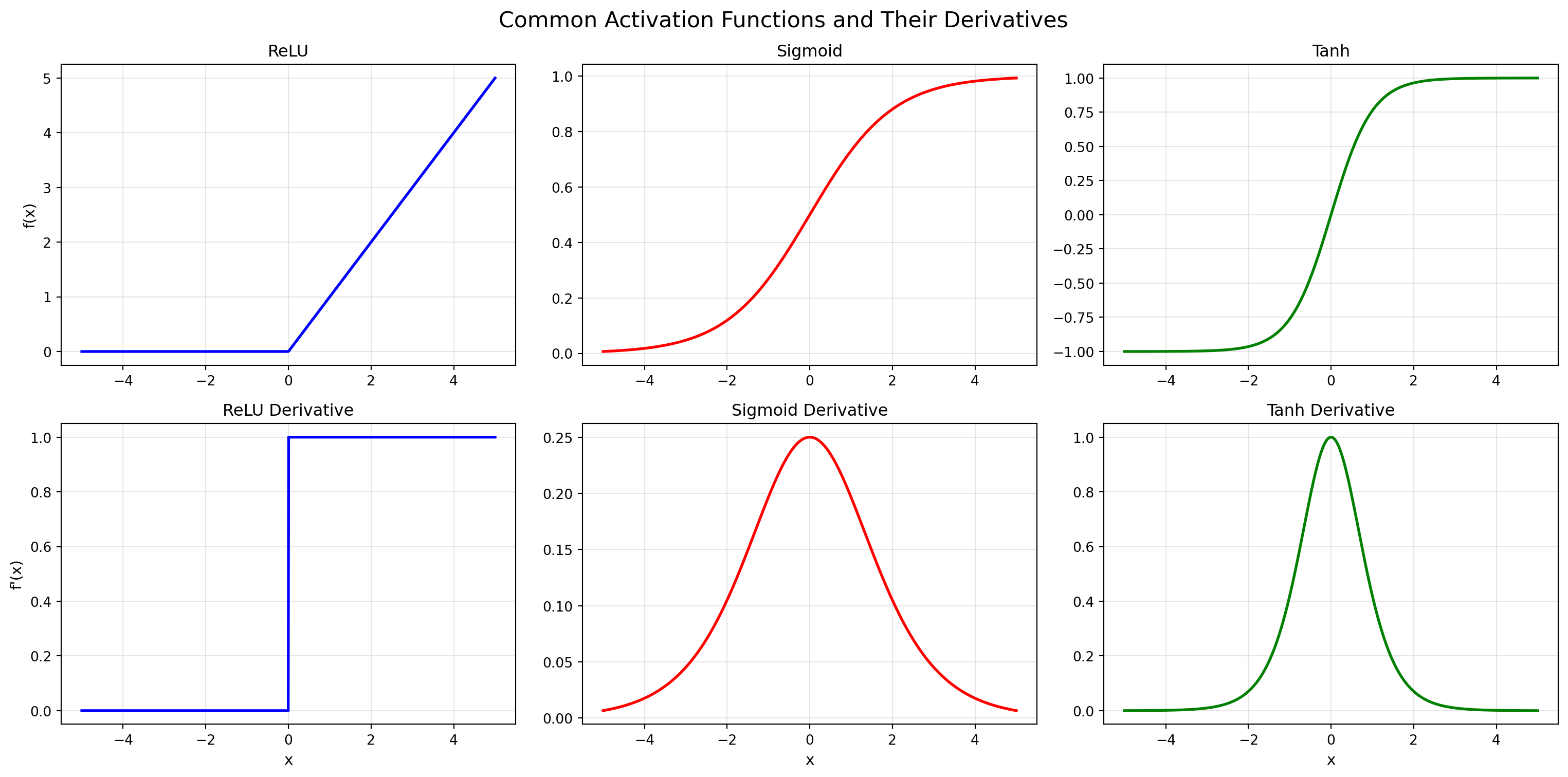
The behavior of an activation function is determined by two things:
1. **Its shape** - how it transforms inputs
2. **Its derivative** - how gradients flow backward during training
### Define Activation Functions
```{python}
def relu(x):
    return np.clip(x, 0, np.inf)

def relu_derivative(x):
    return np.where(x > 0, 1, 0)

def sigmoid(x):
    return 1 / (1 + np.exp(-x))

def sigmoid_derivative(x):
    return sigmoid(x) * (1 - sigmoid(x))

def tanh(x):
    return np.tanh(x)

def tanh_derivative(x):
    return 1 - np.tanh(x)**2
```
### Plot Functions and Derivatives
```{python}
x = np.linspace(-5, 5, 1000)

fig, axes = plt.subplots(2, 3, figsize=(16, 8))
fig.suptitle('Common Activation Functions and Their Derivatives', fontsize=16)

# ReLU
axes[0, 0].plot(x, relu(x), linewidth=2, color='blue')
axes[0, 0].set_title('ReLU', fontsize=12)
axes[0, 0].set_ylabel('f(x)', fontsize=11)
axes[1, 0].plot(x, relu_derivative(x), linewidth=2, color='blue')
axes[1, 0].set_title('ReLU Derivative', fontsize=12)
axes[1, 0].set_ylabel("f'(x)", fontsize=11)
axes[1, 0].set_xlabel('x', fontsize=11)

# Sigmoid
axes[0, 1].plot(x, sigmoid(x), linewidth=2, color='red')
axes[0, 1].set_title('Sigmoid', fontsize=12)
axes[1, 1].plot(x, sigmoid_derivative(x), linewidth=2, color='red')
axes[1, 1].set_title('Sigmoid Derivative', fontsize=12)
axes[1, 1].set_xlabel('x', fontsize=11)

# Tanh
axes[0, 2].plot(x, tanh(x), linewidth=2, color='green')
axes[0, 2].set_title('Tanh', fontsize=12)
axes[1, 2].plot(x, tanh_derivative(x), linewidth=2, color='green')
axes[1, 2].set_title('Tanh Derivative', fontsize=12)
axes[1, 2].set_xlabel('x', fontsize=11)

plt.tight_layout()
plt.show()
```
**Key observations:**
- **ReLU**: $f(x) = \max(0, x)$ - Zero for negative inputs, identity for positive. Derivative is 0 or 1 (simple!).
- **Sigmoid**: $f(x) = \frac{1}{1+e^{-x}}$ - Squashes inputs to $(0, 1)$. Derivative peaks at 0, vanishes at extremes (gradient vanishing problem).
- **Tanh**: $f(x) = \tanh(x)$ - Similar to sigmoid but outputs in $(-1, 1)$. Zero-centered with stronger gradients than sigmoid.
## The Dead ReLU Problem: When Neurons Stop Learning
ReLU's simplicity is its strength, but also its weakness. A ReLU neuron can "die" - permanently outputting zero and never learning again.
**Why does this happen?**
When a neuron's pre-activation values are consistently negative (due to poor initialization, high learning rate, or bad gradients), ReLU outputs zero. Since the derivative is also zero for negative inputs, no gradient flows backward. The neuron is stuck forever.
```{python}
# Generate input data
x = torch.randn(1000, 10)  # 1000 samples, 10 features
linear = nn.Linear(10, 5)   # 5 hidden units

# Set bias to large negative values to "kill" neurons
with torch.no_grad():
    linear.bias.fill_(-10.0)

# Forward pass
pre_activation = linear(x)
post_activation = torch.relu(pre_activation)

# Calculate statistics
dead_percentage = (post_activation == 0).float().mean() * 100
print(f"Percentage of dead neurons: {dead_percentage:.2f}%\n")

# Display table showing ReLU input vs output
print("ReLU Input vs Output (first 10 samples, neuron 0):")
print("-" * 50)
print(f"{'Sample':<10} {'Pre-Activation':<20} {'Post-Activation':<20}")
print("-" * 50)

for i in range(10):
    pre_val = pre_activation[i, 0].item()
    post_val = post_activation[i, 0].item()
    print(f"{i:<10} {pre_val:<20.4f} {post_val:<20.4f}")

print("\nObservation: All negative inputs become 0 after ReLU → Dead neuron!")
```
With a large negative bias, every input becomes negative after the linear transformation. ReLU zeros them all out. The gradient is zero everywhere. The neuron never updates. It's dead.
## Experiment: Do Different Activations Make a Difference?
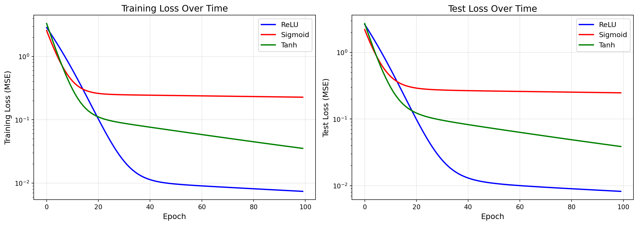
Theory is nice, but let's see activation functions in action. We'll train three identical networks with different activations on a simple regression task: $y = \sin(x) + x^2 + 1$.
### Generate Data
```{python}
# Training data
x_train = np.random.rand(200, 1)
y_train = np.sin(x_train) + np.power(x_train, 2) + 1

# Test data
x_test = np.random.rand(50, 1)
y_test = np.sin(x_test) + np.power(x_test, 2) + 1

# Convert to PyTorch tensors
x_train_tensor = torch.FloatTensor(x_train)
y_train_tensor = torch.FloatTensor(y_train)
x_test_tensor = torch.FloatTensor(x_test)
y_test_tensor = torch.FloatTensor(y_test)
```
### Create and Train Models
```{python}
def create_regression_model(activation_fn):
    """Create a 2-layer network with specified activation"""
    return nn.Sequential(
        nn.Linear(1, 20),
        activation_fn,
        nn.Linear(20, 1)
    )

# Create 3 models with different activations
models = {
    'ReLU': create_regression_model(nn.ReLU()),
    'Sigmoid': create_regression_model(nn.Sigmoid()),
    'Tanh': create_regression_model(nn.Tanh())
}

# Training configuration
n_epochs = 100
learning_rate = 0.01
loss_fn = nn.MSELoss()

# Track metrics
loss_history = {name: [] for name in models.keys()}
test_mse_history = {name: [] for name in models.keys()}

# Train each model
for name, model in models.items():
    optimizer = torch.optim.SGD(model.parameters(), lr=learning_rate)

    for epoch in range(n_epochs):
        # Training
        model.train()
        y_pred = model(x_train_tensor)
        loss = loss_fn(y_pred, y_train_tensor)

        optimizer.zero_grad()
        loss.backward()
        optimizer.step()

        loss_history[name].append(loss.item())

        # Evaluation on test set
        model.eval()
        with torch.no_grad():
            y_test_pred = model(x_test_tensor)
            test_mse = loss_fn(y_test_pred, y_test_tensor).item()
            test_mse_history[name].append(test_mse)
```
### Compare Learning Curves
```{python}
fig, axes = plt.subplots(1, 2, figsize=(14, 5))
colors = {'ReLU': 'blue', 'Sigmoid': 'red', 'Tanh': 'green'}

# Plot training loss
for name, losses in loss_history.items():
    axes[0].plot(losses, label=name, linewidth=2, color=colors[name])

axes[0].set_xlabel('Epoch', fontsize=12)
axes[0].set_ylabel('Training Loss (MSE)', fontsize=12)
axes[0].set_title('Training Loss Over Time', fontsize=14)
axes[0].legend(fontsize=11)
axes[0].grid(True, alpha=0.3)
axes[0].set_yscale('log')

# Plot test MSE
for name, test_mse in test_mse_history.items():
    axes[1].plot(test_mse, label=name, linewidth=2, color=colors[name])

axes[1].set_xlabel('Epoch', fontsize=12)
axes[1].set_ylabel('Test Loss (MSE)', fontsize=12)
axes[1].set_title('Test Loss Over Time', fontsize=14)
axes[1].legend(fontsize=11)
axes[1].grid(True, alpha=0.3)
axes[1].set_yscale('log')

plt.tight_layout()
plt.show()

# Print final metrics
print("\nFinal Metrics after {} epochs:".format(n_epochs))
print("-" * 60)
print(f"{'Activation':<15} {'Train Loss':<15} {'Test Loss':<15}")
print("-" * 60)
for name in models.keys():
    train_loss = loss_history[name][-1]
    test_loss = test_mse_history[name][-1]
    print(f"{name:<15} {train_loss:<15.6f} {test_loss:<15.6f}")
```

