Goodfellow Deep Learning — Chapter 8.3: Basic Algorithms
Stochastic Gradient Descent
Stochastic Gradient Descent (SGD) is the most fundamental optimization algorithm in deep learning. Unlike batch gradient descent, which computes gradients over the entire training set, SGD uses small random samples (minibatches) to estimate the gradient, making it computationally efficient for large datasets.
Algorithm
Hyperparameters:
- Learning rate \(\epsilon\)
- Initial parameters \(\theta\)
Training procedure:
While stopping criterion not met, do:
- Sample a minibatch of m examples from the training set
- Compute the loss and gradient on the minibatch
- Compute the gradient estimate:
\[ \hat{g} \leftarrow +\frac{1}{m}\nabla_{\theta}\sum_i L(f(x^{(i)};\theta), y^{(i)}) \]
- Update parameters:
\[ \theta \leftarrow \theta - \epsilon \hat{g} \]
Sufficient Conditions for Convergence
A critical question in SGD is: how should we choose the learning rate schedule to guarantee convergence? For SGD to converge to a minimum, the learning rate schedule must satisfy two complementary conditions that balance exploration and stability:
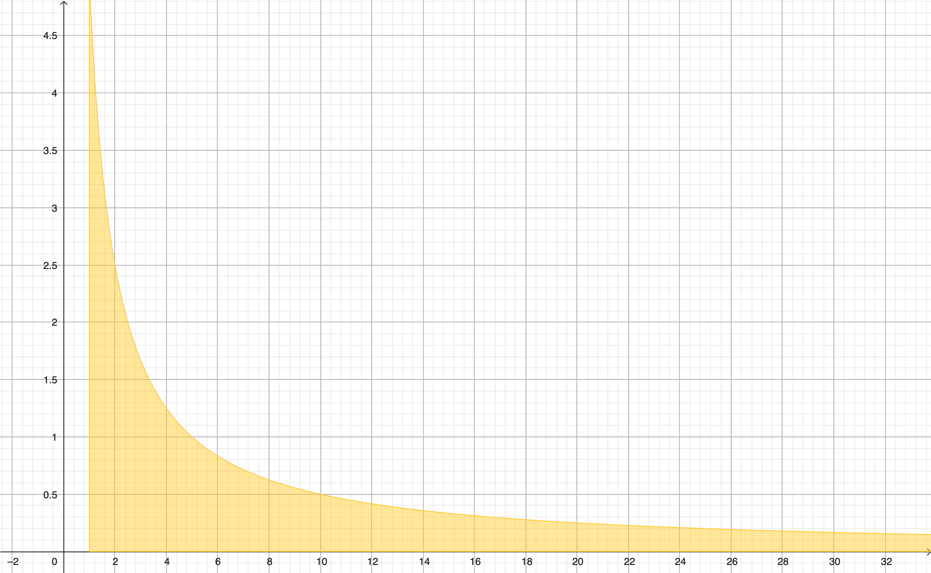
Condition 1: The sum of learning rates must diverge (equation 8.12):
\[ \sum_{k=1}^{\infty}\epsilon_k = \infty \tag{8.12} \]
In other words, \(\epsilon_1 + \epsilon_2 + \ldots\) must be unbounded.

This condition ensures that the algorithm can reach any point in parameter space, no matter how far from the initialization.
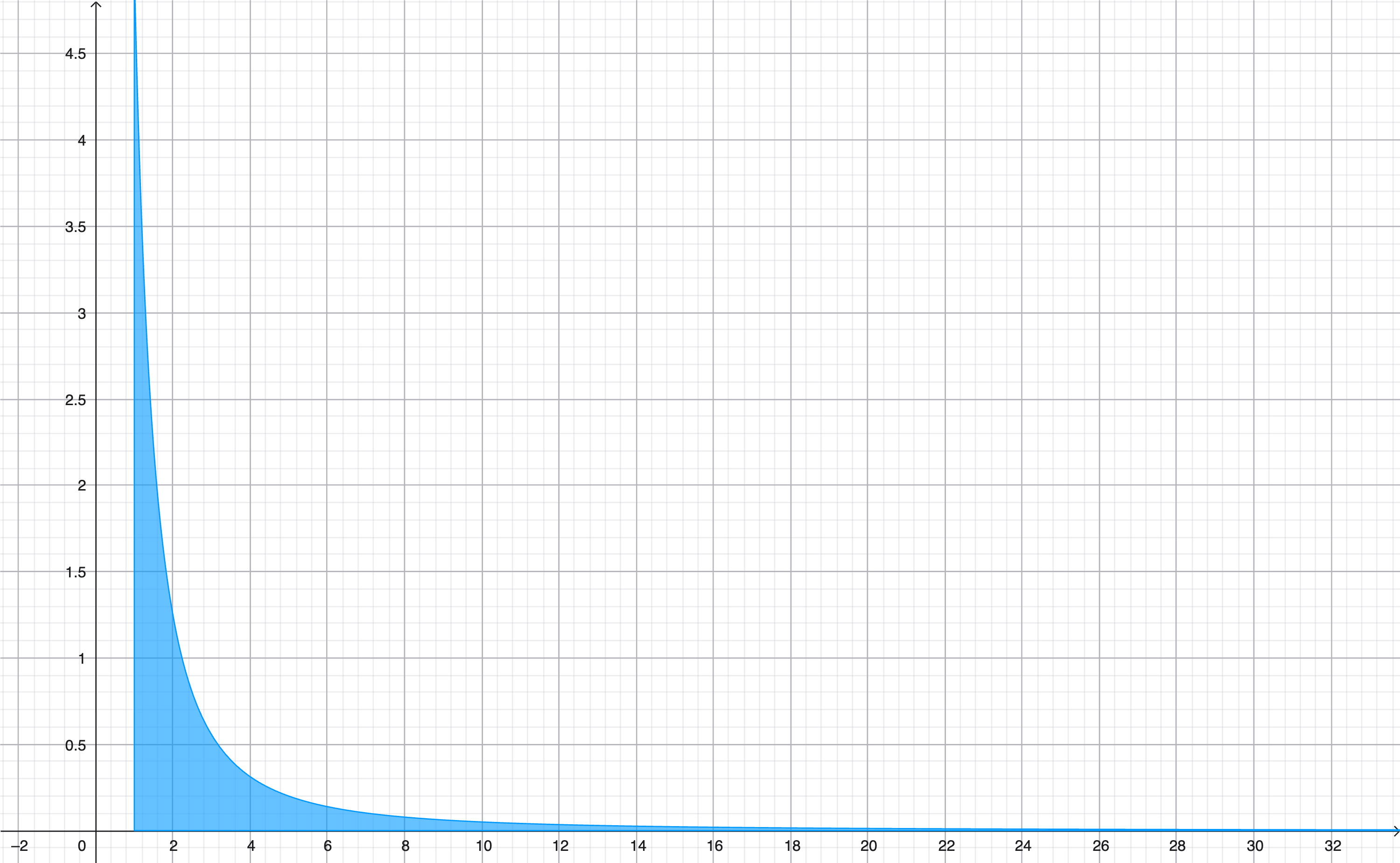
Condition 2: The sum of squared learning rates must converge (equation 8.13):
\[ \sum_{k=1}^{\infty} \epsilon_k^2 < \infty \tag{8.13} \]
In other words, \(\epsilon_1^2 + \epsilon_2^2 + \ldots = C\) (a finite constant).

This condition ensures that the accumulated noise from stochastic gradient estimates remains bounded, allowing the algorithm to settle into a minimum rather than bouncing around indefinitely.
Summary: Together, these two conditions ensure that SGD can initially make large steps to explore parameter space (Condition 1), while eventually taking smaller steps that allow convergence to a minimum (Condition 2).
Practical Learning Rate Scheduling: Linear Decay
While the theoretical conditions above provide convergence guarantees, they are often impractical for real-world training.
A commonly used learning rate schedule in practice is linear decay (equation 8.14):
\[ \epsilon_k = (1-\alpha)\epsilon_0 + \alpha \epsilon_{\tau} \tag{8.14} \]
where \(\alpha = \frac{k}{\tau}\).
This schedule starts at \(\epsilon_0\) and linearly decreases to \(\epsilon_{\tau}\) over \(\tau\) iterations. After \(\tau\) iterations, when \(\alpha = 1\), the learning rate remains fixed at \(\epsilon_{\tau}\).
Momentum
While SGD provides a solid foundation for optimization, it can struggle with ill-conditioned loss surfaces where gradients in different directions have vastly different magnitudes. Momentum addresses this problem by adding “inertia” to parameter updates. It accelerates learning in directions with consistent gradients and smooths oscillations in steep or noisy directions.
The momentum method introduces a velocity variable \(v\) that accumulates an exponentially decaying moving average of past gradients:
\[ v_t = \beta v_{t-1} + (1-\beta)\nabla_\theta L(\theta) \]
\[ \theta_{t+1} = \theta_t - \epsilon v_t \]
where:
- \(\beta\) is the momentum coefficient (typically 0.9)
- \(v_t\) is the velocity, representing the weighted average of gradients
- \(\epsilon\) is the learning rate
Alternative Formulation
The momentum algorithm can equivalently be written in a slightly different form (equations 8.15-8.16):
\[ v \leftarrow \alpha v - \epsilon \nabla_\theta \left(\frac{1}{m}\sum_{i=1}^m L(f(x^{(i)}; \theta), y^{(i)}) \right) \tag{8.15} \]
\[ \theta \leftarrow \theta + v \tag{8.16} \]
In this formulation, \(\epsilon\) represents the learning rate scaled by \((1-\alpha)\). Note that here we use \(\alpha\) instead of \(\beta\) as the momentum coefficient, and the parameter update adds the velocity instead of subtracting it.
Maximum Step Length
Equation 8.17 gives the upper bound of the effective step size in momentum-based SGD:
\[ \text{Max step length} = \frac{\epsilon \lVert g \rVert}{1 - \alpha} \tag{8.17} \]
Intuition: Assuming the gradients \(g_t\) remain in a consistent direction, the velocity accumulates geometrically as:
\[ v_t = -\epsilon(g_t + \alpha g_{t-1} + \alpha^2 g_{t-2} + \cdots) \]
which converges to \(\frac{\epsilon g}{1 - \alpha}\).
This shows that momentum effectively amplifies the step length by a factor of \(\frac{1}{1-\alpha}\).
Example: With \(\alpha = 0.9\), the effective speed can be up to 10× faster than standard SGD.
Physical Interpretation: Newton’s Law of Acceleration
The momentum method is not just a mathematical trick — it has a deep connection to classical physics. We can understand momentum optimization by drawing an analogy with a particle moving on a physical surface under the influence of forces.
Equation 8.18 - Newton’s Second Law of Motion:
In physics, force equals mass times acceleration:
\[ F = ma = m\frac{\partial^2 x}{\partial t^2} \]
In deep learning, assuming \(m = 1\) and viewing the parameters \(\theta\) as the position of a particle on the loss surface, we obtain:
\[ f(t) = \frac{\partial^2 \theta(t)}{\partial t^2} \tag{8.18} \]
This expresses that the force acting on parameters corresponds to their acceleration, forming the physical foundation of momentum optimization.
Equation 8.19 - Velocity as Rate of Change:
To further express the relationship between force, velocity, and position, we define velocity \(v(t)\) as the first derivative of the position \(\theta(t)\) with respect to time:
\[ v(t) = \frac{\partial \theta(t)}{\partial t} \tag{8.19} \]
\[ f(t) = \frac{\partial v(t)}{\partial t} \]
The velocity is the instantaneous rate of change — the first derivative of position. Likewise, the force (or acceleration) is the instantaneous rate of change of velocity — the first derivative of velocity.
This physical interpretation helps us understand why momentum works: the negative gradient acts as a force pushing the parameters downhill, while the velocity variable accumulates this force over time, allowing the optimizer to build up speed in consistent directions.
Damping in Momentum
In the physical analogy, we can also understand the momentum coefficient \(\alpha\) as a damping or friction term that prevents the optimizer from accelerating indefinitely.
In momentum optimization, the damping (or friction) effect is implicitly controlled by the factor \(\alpha\) in the velocity update rule:
\[ v_t = \alpha v_{t-1} - \epsilon \nabla_\theta L(\theta_t) \]
This formulation can be seen as a discrete version of Newton’s second law with viscous damping:
\[ \frac{d^2 \theta}{dt^2} = -\nabla_\theta L(\theta) - \mu \frac{d\theta}{dt} \]
where the damping coefficient \(\mu\) corresponds to \(1 - \alpha\).
Intuition:
- \(\alpha\) determines how much of the previous velocity is retained (the inertia)
- \(1 - \alpha\) represents the proportion of velocity lost due to friction
Effect of \(\alpha\):
- When \(\alpha\) is close to 1 (e.g., 0.99), damping is weak — the optimizer moves faster but tends to oscillate near minima
- When \(\alpha\) is smaller (e.g., 0.5), damping is strong — the motion is smoother but slower
Nesterov Momentum
While standard momentum provides significant improvements over vanilla SGD, it still has a limitation: it computes gradients at the current position without considering where the momentum will take us next. Nesterov momentum addresses this by introducing a “lookahead” mechanism.
Standard momentum looks backward — it uses gradients from the current position. Nesterov momentum looks ahead — it first predicts the next position \(\theta + \alpha v\) and then calculates the gradient there.
This leads to the modified update rule (equation 8.21):
\[ v_{t+1} = \alpha v_t - \epsilon \nabla_\theta L(\theta_t + \alpha v_t) \]
\[ v \leftarrow \alpha v - \epsilon \nabla_{\theta}\left[\frac{1}{m} \sum_{i=1}^m L(f(x^{(i)};\theta + \alpha v), y^{(i)}) \right] \tag{8.21} \]
Finally, the parameters are updated using this new velocity (equation 8.22):
\[ \theta_{t+1} = \theta_t + v_{t+1} \tag{8.22} \]
This “lookahead” strategy allows the optimizer to anticipate its next move, resulting in faster convergence and less oscillation near minima compared to standard momentum.
Intuition: Imagine you’re rolling a ball down a hill. Standard momentum uses the slope at your current position to decide how fast to roll. Nesterov momentum is smarter — it first looks ahead to where the momentum will carry you, checks the slope there, and then adjusts the velocity accordingly. This prevents overshooting and makes the optimizer more responsive to the local curvature of the loss surface.