Goodfellow Deep Learning — Chapter 7.8: Early Stopping
Overview
Early stopping is a simple yet effective regularization technique that stops training when validation performance begins to degrade.
1. The Overfitting Problem

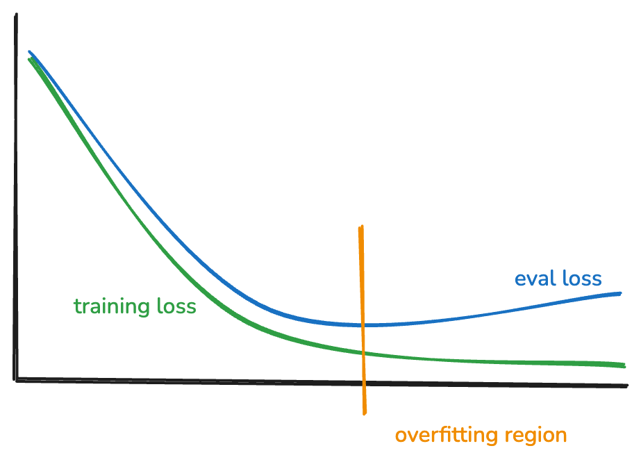
Observation: Overfitting almost always occurs during training.
What happens:
- Training error continues to decrease
- Validation error initially decreases, then starts increasing
- The gap between training and validation error grows
- Model memorizes training data instead of learning generalizable patterns
Solution: Stop training when validation error reaches its minimum.
2. Two Approaches to Early Stopping
Split data into training \((x, y)\) and validation \((x_{\text{valid}}, y_{\text{valid}})\):
Approach 1: Find Optimal Steps, Then Retrain
- Train on \((x, y)\) while monitoring \(y_{\text{valid}}\)
- Identify the optimal number of steps \(\tau^*\) where validation error is minimized
- Retrain from scratch on full dataset for exactly \(\tau^*\) steps
Advantage: Uses all data for final training
Disadvantage: Requires two full training runs
Approach 2: Keep Best Model
- Train on \((x, y)\) while monitoring \(y_{\text{valid}}\)
- Keep a copy of the model whenever validation performance improves
- Stop when validation error stops improving
- Use the saved best model
Advantage: Only requires one training run
Disadvantage: Validation data is not used for training

3. Costs of Early Stopping
Data requirements:
- Need to hold out a portion of data as validation set
- Reduces effective training data size
- Validation set typically 10-20% of total data
Computational requirements:
- Need to keep a copy of the best-performing model
- Requires periodic evaluation on validation set
- May need multiple checkpoints if using approach 1
4. Benefits of Early Stopping
Regularization:
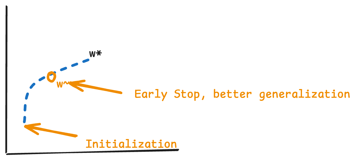
- Prevents overfitting without modifying the loss function
- Acts as implicit L2 regularization (proven mathematically below)
- No hyperparameter tuning needed for regularization strength
Efficiency:
- Saves computation by stopping early
- Automatic hyperparameter selection (number of iterations)
- Often faster than training with explicit regularization to convergence
Simplicity:
- Easy to implement
- Widely applicable across different model types
- Works well in practice without fine-tuning
5. Mathematical Connection to L2 Regularization
Gradient Descent Update Rule
Starting from a quadratic approximation around the optimal weights \(w^*\):
Equation 7.33 - Quadratic approximation of loss:
\[ \hat{J}(\theta) = J(w^*) + \frac{1}{2}(w - w^*)^T H(w - w^*) \]
where \(H\) is the Hessian matrix at \(w^*\).
Equation 7.34 - Gradient:
\[ \nabla_w \hat{J}(w) = H(w - w^*) \]
Equation 7.35 - Gradient descent update:
\[ w^{(\tau)} = w^{(\tau-1)} - \epsilon \nabla_w \hat{J}(w^{(\tau-1)}) \]
Equation 7.36 - Substituting the gradient:
\[ w^{(\tau)} = w^{(\tau-1)} - \epsilon H(w^{(\tau-1)} - w^*) \]
Equation 7.37 - Rearranging:
\[ w^{(\tau)} - w^* = (I - \epsilon H)(w^{(\tau-1)} - w^*) \]
Eigendecomposition of Hessian
Equation 7.38 - Decompose \(H = Q\Lambda Q^T\):
\[ w^{(\tau)} - w^* = (I - \epsilon Q\Lambda Q^T)(w^{(\tau-1)} - w^*) \]
Equation 7.39 - Multiply both sides by \(Q^T\):
\[ Q^T(w^{(\tau)} - w^*) = (I - \epsilon \Lambda)Q^T(w^{(\tau-1)} - w^*) \]
Deriving the Recursive Formula
Since \((I - \epsilon\Lambda)\) is a constant diagonal matrix, we can apply this recursion:
Step 1 - After 1 iteration:
\[ Q^T(w^{(1)} - w^*) = (I - \epsilon \Lambda)Q^T(w^{(0)} - w^*) \]
Step 2 - After 2 iterations:
\[ \begin{aligned} Q^T(w^{(2)} - w^*) &= (I - \epsilon \Lambda)Q^T(w^{(1)} - w^*) \\ &= (I - \epsilon \Lambda)Q^T(I - \epsilon \Lambda)(w^{(0)} - w^*) \\ &= (I - \epsilon \Lambda)^2 Q^T(w^{(0)} - w^*) \end{aligned} \]
Step 3 - After 3 iterations:
\[ \begin{aligned} Q^T(w^{(3)} - w^*) &= (I - \epsilon \Lambda)Q^T(w^{(2)} - w^*) \\ &= (I - \epsilon \Lambda)Q^T(I - \epsilon \Lambda)^2(w^{(0)} - w^*) \\ &= (I - \epsilon \Lambda)^3 Q^T(w^{(0)} - w^*) \end{aligned} \]
General pattern - After \(\tau\) iterations:
\[ Q^T(w^{(\tau)} - w^*) = (I - \epsilon \Lambda)^\tau Q^T(w^{(0)} - w^*) \]
Assuming Zero Initialization
Equation 7.40 - If \(w^{(0)} = 0\):
\[ \begin{aligned} Q^T(w^{(\tau)} - w^*) &= (I - \epsilon \Lambda)^\tau Q^T(0 - w^*) \\ &= -(I - \epsilon \Lambda)^\tau Q^T w^* \end{aligned} \]
Therefore:
\[ Q^T w^{(\tau)} = Q^T w^* - (I - \epsilon \Lambda)^\tau Q^T w^* \]
\[ Q^T w^{(\tau)} = [I - (I - \epsilon \Lambda)^\tau] Q^T w^* \]
L2 Regularization Solution
Equation 7.41 - L2 regularized solution:
\[ Q^T \tilde{w} = (\Lambda + \alpha I)^{-1} \Lambda Q^T w^* \]
Equation 7.42 - Rewriting:
\[ Q^T \tilde{w} = [I - (\Lambda + \alpha I)^{-1} \alpha] Q^T w^* \]
Equivalence Condition
Equation 7.43 - Comparing equations 7.40 and 7.42:
If we can set:
\[ (I - \epsilon \Lambda)^\tau = (\Lambda + \alpha I)^{-1} \alpha \]
then early stopping is equivalent to L2 regularization.
6. Relationship Between Training Steps and Regularization Strength
Deriving \(\tau\) from \(\alpha\)
Mathematical tools:
- Logarithm properties: \(\log(ab) = \log(a) + \log(b)\) and \(\log(a^b) = b\log(a)\)
- Taylor series approximation: \(\log(1 + x) \approx x\) and \(\log(1 - x) \approx -x\)
Starting from equation 7.43:
\[ \tau \log(I - \epsilon \Lambda) = \log((\Lambda + \alpha I)^{-1} \alpha) \]
Right side:
\[ \log((\Lambda + \alpha I)^{-1} \alpha) = -\log(\Lambda + \alpha I) + \log(\alpha) \]
Factor out \(\alpha\):
\[ \Lambda + \alpha I = \alpha\left(\frac{\Lambda}{\alpha} + I\right) \]
Therefore:
\[ -\log(\Lambda + \alpha I) + \log(\alpha) = -\log(\alpha) - \log\left(\frac{\Lambda}{\alpha} + I\right) + \log(\alpha) = -\log\left(\frac{\Lambda}{\alpha} + I\right) \]
Left side using Taylor approximation:
\[ \log(I - \epsilon \Lambda) \approx -\epsilon \Lambda \]
Right side using Taylor approximation:
\[ \log\left(I + \frac{\Lambda}{\alpha}\right) \approx \frac{\Lambda}{\alpha} \]
Combining:
\[ \tau(-\epsilon \Lambda) \approx -\frac{\Lambda}{\alpha} \]
Equation 7.44 - Solving for \(\tau\):
\[ \tau \approx \frac{1}{\epsilon \alpha} \]
Equation 7.45 - Solving for \(\alpha\):
\[ \alpha \approx \frac{1}{\epsilon \tau} \]
Key Insight
The number of training steps \(\tau\) is inversely proportional to the L2 regularization strength \(\alpha\).
Interpretation:
- More training steps (\(\tau\) large) ↔︎ Weaker regularization (\(\alpha\) small)
- Fewer training steps (\(\tau\) small) ↔︎ Stronger regularization (\(\alpha\) large)
- Early stopping implicitly applies L2 regularization with strength \(\alpha \approx \frac{1}{\epsilon \tau}\)
Practical implication: Choosing when to stop training is equivalent to choosing the regularization strength.
Key concepts:
- Early stopping: Stop training when validation error stops improving
- Two approaches: Find optimal steps and retrain, or keep best model
- Costs: Requires validation data and model checkpointing
- Benefits: Simple, effective, computationally efficient regularization
- Mathematical equivalence: Early stopping ≈ implicit L2 regularization
- Inverse relationship: \(\tau \approx \frac{1}{\epsilon \alpha}\) (more steps = less regularization)
Source: Deep Learning Book, Chapter 7.8