MIT 18.06 Lecture 16: Projection Matrices and Least Squares
This lecture builds on Lecture 15: Projection onto Subspaces, where we derived the projection formula and normal equations.
Projection Matrix
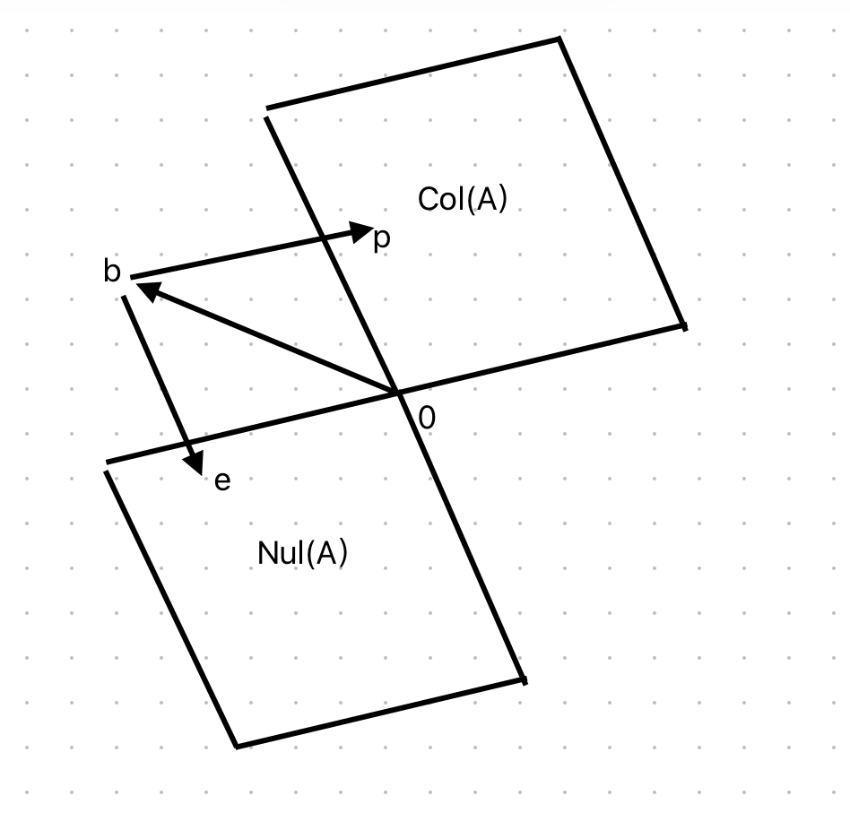
The projection matrix \(P\) projects any vector \(b\) onto the column space of \(A\).
\[ P=A(A^\top A)^{-1}A^\top \]
Key properties:
- If \(b\) is in the column space, \(Pb=b\)
- If \(b\) is perpendicular to the column space, \(Pb=0\)

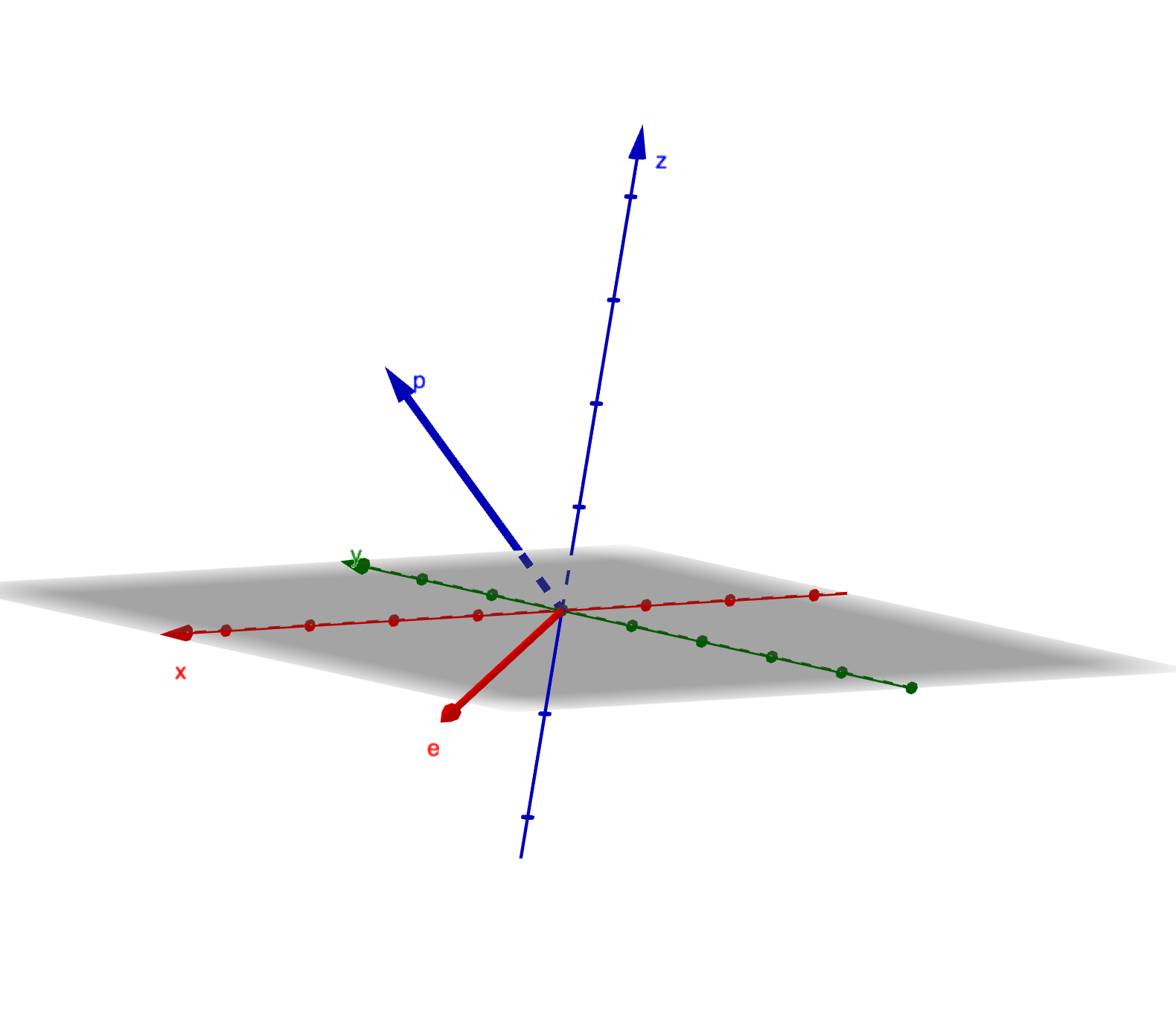
\[ p+e=b \]
\[ \begin{aligned} Pb &= p \\ e &= (I-P)b \end{aligned} \]
Orthogonal decomposition:
- \(p\) is in the column space
- \(e\) is in the left null space
This decomposition shows that any vector \(b\) can be split into its projection \(p\) and error \(e\), which are orthogonal.
Least Squares
When \(Ax=b\) has no solution, least squares finds the \(x\) that minimizes the error \(\|Ax-b\|\).

Setup:
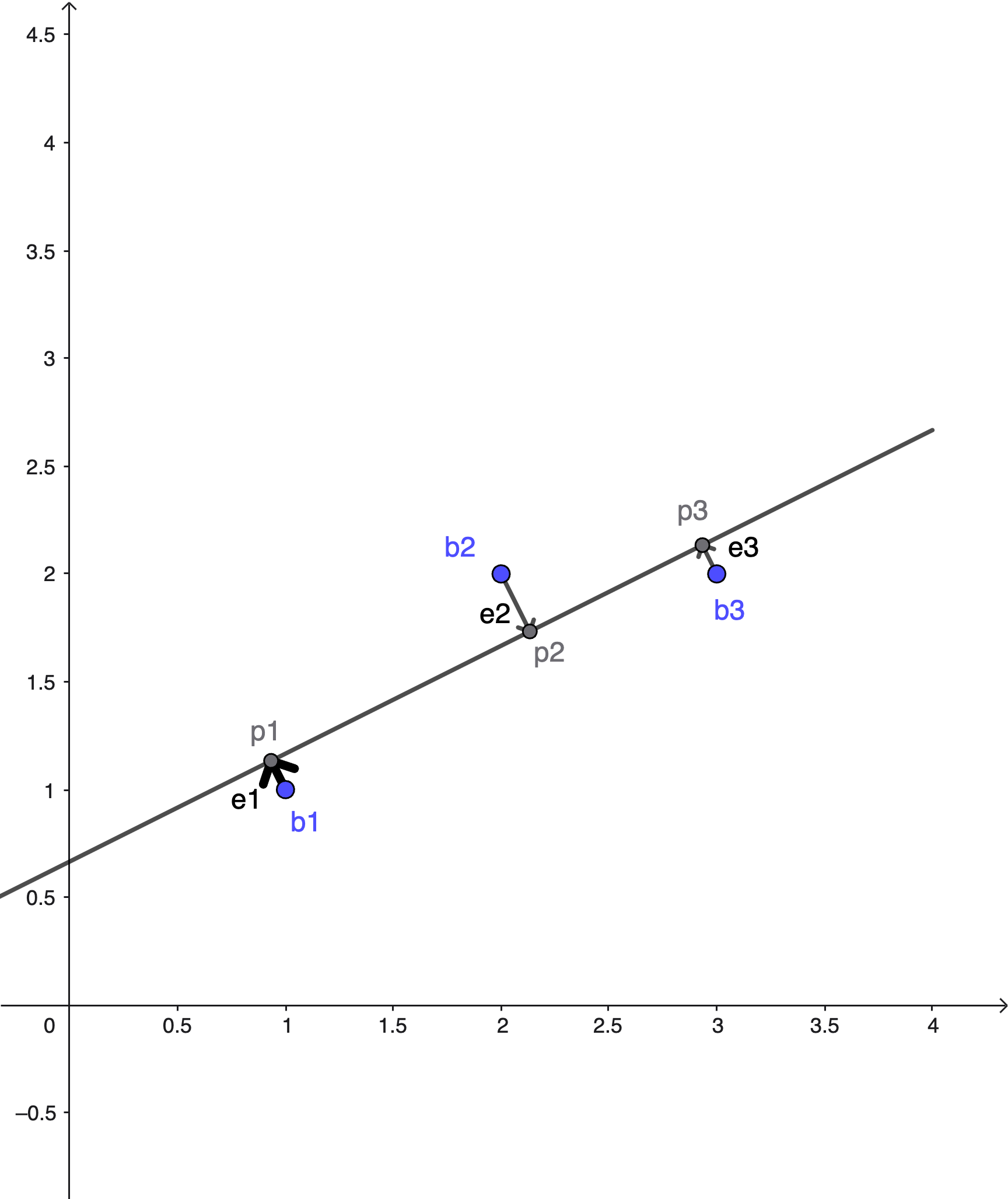
- \(b_1, b_2, b_3\) are not on the same line, so we cannot solve \(Ax=b\) exactly
- \(p_1, p_2, p_3\) are on the same line - the best fit line
Objective:
\[ \arg\min\|Ax-b\|^2 = e_1^2+e_2^2+e_3^2 \]
Example: Fit a line \(C+Dt\) to points \((1,1)\), \((2,2)\), \((3,2)\):
\[ \begin{aligned} C+D &= 1 \\ C+2D &= 2 \\ C+3D &= 2 \end{aligned} \]
This is the equation \(Ax=b\):
\[ \begin{bmatrix}1&1\\1&2\\1&3\end{bmatrix} \begin{bmatrix}C\\D\end{bmatrix}=\begin{bmatrix}1\\2\\2\end{bmatrix} \]
Finding the Best Fit
Goals:
- Find \(\hat{x}=\begin{bmatrix}\hat{C}\\\hat{D}\end{bmatrix}\), the best fit line (not the perfect line)
- Find the projection \(P\)
Normal equation:
\[ A^\top A\hat{x}=A^\top b \]
This is called the normal equation because \(A^\top(A\hat{x}-b)=0\) means the error is normal (perpendicular) to the column space.
Computation:
\(A^\top A\):
\[ \begin{bmatrix}1&1&1\\1&2&3\end{bmatrix}\begin{bmatrix}1&1\\1&2\\1&3\end{bmatrix} =\begin{bmatrix}3&6\\6&14\end{bmatrix} \]
\(A^\top b\):
\[ \begin{bmatrix}1&1&1\\1&2&3\end{bmatrix}\begin{bmatrix}1\\2\\2\end{bmatrix}=\begin{bmatrix}5\\11\end{bmatrix} \]
System:
\[ \begin{aligned} 3C+6D &= 5 \\ 6C+14D &= 11 \end{aligned} \]
Solution: \(C=\frac{2}{3}\), \(D=\frac{1}{2}\)
Calculating Projections and Errors
Projections:
- \(p_1=\frac{2}{3}+\frac{1}{2}=\frac{7}{6}\)
- \(p_2=\frac{2}{3}+1=\frac{5}{3}\)
- \(p_3=\frac{2}{3}+\frac{3}{2}=\frac{13}{6}\)
Errors:
- \(e_1=1-\frac{7}{6}=-\frac{1}{6}\)
- \(e_2=2-\frac{5}{3}=\frac{1}{3}\)
- \(e_3=2-\frac{13}{6}=-\frac{1}{6}\)
Verify perpendicularity:
- \(p=\begin{bmatrix}\frac{7}{6}\\\frac{5}{3}\\\frac{13}{6}\end{bmatrix}\)
- \(e=\begin{bmatrix}-\frac{1}{6}\\\frac{1}{3}\\-\frac{1}{6}\end{bmatrix}\)

Preview: Orthonormal Matrices
This is a preview for the next lecture.
The vectors \([0,0,1]\), \([0,1,0]\), \([1,0,0]\) are orthonormal unit vectors (perpendicular to each other with unit length).
If we arrange them as columns in matrix \(Q\):
\[ Q^\top Q=I_n \]
Another orthonormal matrix: The rotation matrix:
\[ \begin{bmatrix}\cos\theta&-\sin\theta\\\sin\theta &\cos\theta\end{bmatrix} \]
Proof that columns are unit vectors:
- \((\cos\theta)^2+(\sin\theta)^2=1\)
- \((-\sin\theta)^2+(\cos\theta)^2=1\)
Proof of perpendicularity:
- \(q_1^\top q_2 = \cos\theta(-\sin\theta) + \sin\theta(\cos\theta) = 0\)
Connection to Calculus
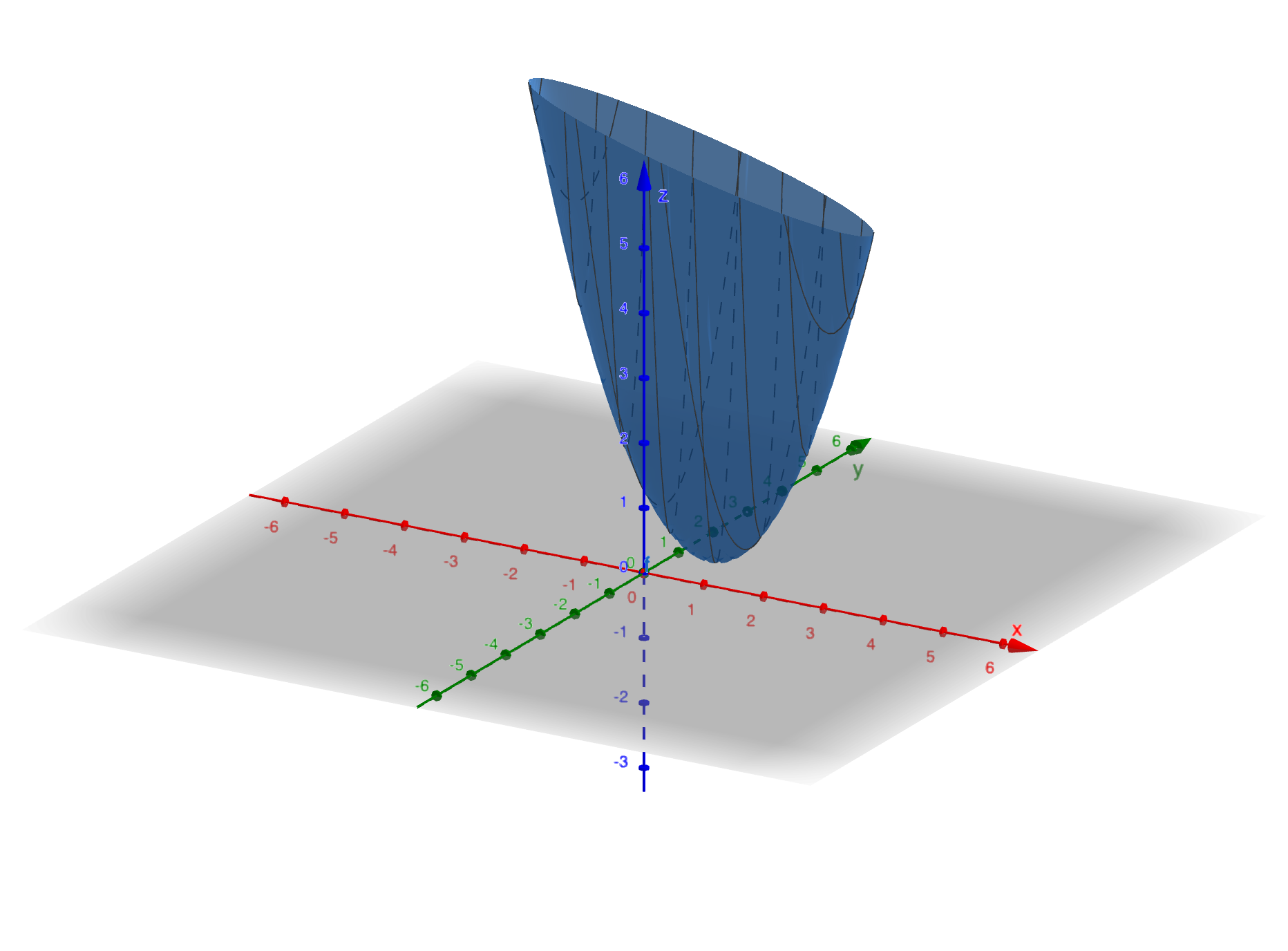
From the error minimization perspective, we have the error function:
\[ (C+D-1)^2+(C+2D-2)^2+(C+3D-2)^2 \]

We can find the minimum by setting the gradient to zero for this positive definite function.
The professor briefly introduced this approach to show the connection between linear algebra and calculus.
Source: MIT 18.06SC Linear Algebra, Lecture 16