MIT 18.06 Lecture 27: Positive Definite Matrices and Minima
This lecture deepens our understanding of positive definite matrices by connecting them to multivariable calculus, optimization, and geometry. We explore how these matrices guarantee the existence of unique minima and how their eigenvalues shape the geometry of quadratic forms.
Review: Tests for Positive Definiteness
A symmetric matrix \(A\) is positive definite if any of the following equivalent conditions hold:
1. Energy Test
\[ x^{\top}Ax > 0 \quad \text{for all } x \neq 0 \]
2. Eigenvalue Test
All eigenvalues are positive: \(\lambda_i > 0\) for all \(i\)
3. Pivot Test
All pivots are positive (from Gaussian elimination)
4. Determinant Test
All leading principal minors have positive determinants: - \(\det(A_1) > 0\) - \(\det(A_2) > 0\) - \(\vdots\) - \(\det(A_n) > 0\)
where \(A_k\) is the upper-left \(k \times k\) submatrix.
Example: 2×2 Positive Definite Matrix
Consider: \[ A = \begin{bmatrix}a & b \\ b & c\end{bmatrix} \]
Tests for positive definiteness:
Determinants:
- \(a > 0\) (first principal minor)
- \(ac - b^2 > 0\) (full determinant)
Pivots:
- First pivot: \(a > 0\)
- Second pivot: \(\frac{ac - b^2}{a} > 0\)
Eigenvalues: Both \(\lambda_1 > 0\) and \(\lambda_2 > 0\)
Energy: \(x^{\top}Ax > 0\) for all \(x \neq 0\)
Positive Semidefinite Matrices
A matrix is positive semidefinite if \(x^{\top}Ax \geq 0\) for all \(x\) (allowing zero).
Example
\[ A = \begin{bmatrix}2 & 6 \\ 6 & 18\end{bmatrix} \]
Check the tests: - Determinant: \((2 \times 18) - (6 \times 6) = 36 - 36 = 0\) - Eigenvalues: \(\lambda_1 = 0\), \(\lambda_2 = 20\) - Pivots: \(2, 0\)
Since one eigenvalue is zero and the determinant is zero, this matrix is positive semidefinite (not positive definite).
Quadratic Form
\[ x^{\top}Ax = \begin{bmatrix}x_1 & x_2\end{bmatrix}\begin{bmatrix}2 & 6 \\ 6 & 18\end{bmatrix}\begin{bmatrix}x_1 \\ x_2\end{bmatrix} \]
\[ = 2x_1^2 + 12x_1x_2 + 18x_2^2 = 2(x_1 + 3x_2)^2 \geq 0 \]
Key observation: The quadratic form is a perfect square, so it’s always non-negative but can be zero (when \(x_1 = -3x_2\)).

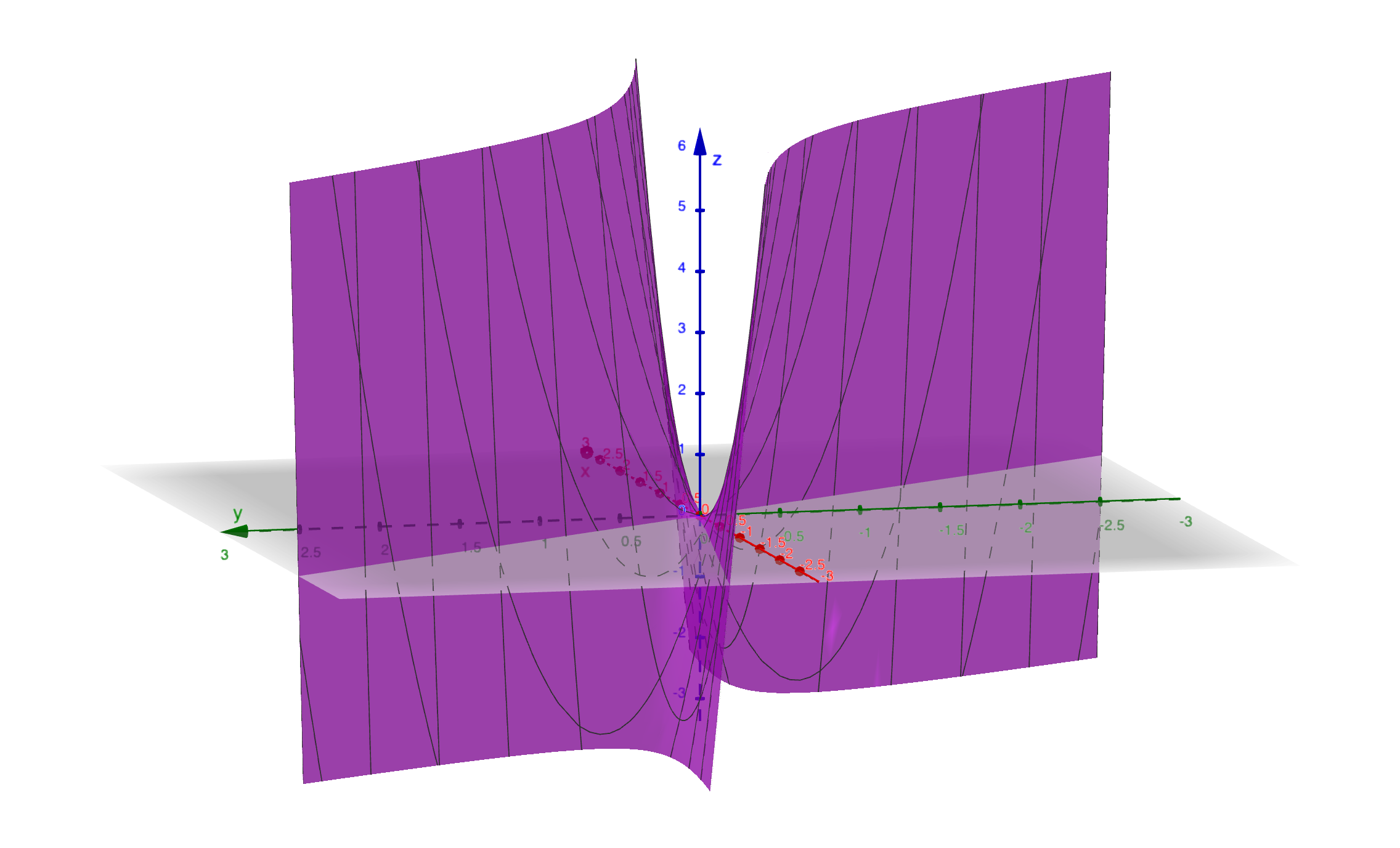
Geometric interpretation: The level curves form a parabolic cylinder—there’s a whole line of minima along \(x_1 + 3x_2 = 0\).
Indefinite Matrices
A matrix is indefinite if \(x^{\top}Ax\) can be both positive and negative depending on \(x\).
Example
\[ A = \begin{bmatrix}2 & 6 \\ 6 & 7\end{bmatrix} \]
Quadratic form: \[ f(x, y) = 2x^2 + 12xy + 7y^2 \]
Finding negative values: - Try \(x = -1, y = 1\): \(f(-1, 1) = 2 - 12 + 7 = -3 < 0\) - Try \(x = 1, y = -1\): \(f(1, -1) = 2 - 12 + 7 = -3 < 0\)
Since the quadratic form can be negative, the matrix is indefinite.
Factorizing the Quadratic Form
We can complete the square: \[ f(x, y) = 2x^2 + 12xy + 7y^2 = 2(x + 3y)^2 - 11y^2 \]
Interpretation: - The term \(2(x + 3y)^2\) is positive - The term \(-11y^2\) is negative - The function has a saddle point at the origin

Geometric interpretation: The surface is a hyperbolic paraboloid (saddle). At the critical point, first-order derivatives are zero, but the function has no minimum—it goes up in some directions and down in others.
Positive Definite Example
Consider: \[ A = \begin{bmatrix}2 & 2 \\ 2 & 20\end{bmatrix} \]
Quadratic form: \[ f(x, y) = 2x^2 + 4xy + 20y^2 \]
Finding the Minimum
Critical point: At the minimum, all partial derivatives must be zero: \[ \frac{\partial f}{\partial x} = 4x + 4y = 0 \] \[ \frac{\partial f}{\partial y} = 4x + 40y = 0 \]
The only solution is \((x, y) = (0, 0)\).
Second derivative test: Computing the second derivatives: \[ \frac{\partial^2 f}{\partial x^2} = 4, \quad \frac{\partial^2 f}{\partial x \partial y} = 4, \quad \frac{\partial^2 f}{\partial y^2} = 40 \]
The Hessian matrix is: \[ H = \begin{bmatrix}4 & 4 \\ 4 & 40\end{bmatrix} = 2A \]
Since \(H = 2A\) is positive definite (all eigenvalues positive, or equivalently \(A\) is positive definite), this confirms \((0, 0)\) is a minimum.
Factorizing the Quadratic Form
Complete the square: \[ f(x, y) = 2x^2 + 4xy + 20y^2 = 2(x + y)^2 + 18y^2 \]
Key insight: Both terms are squares with positive coefficients, so \(f(x, y) \geq 0\) with equality only at \((0, 0)\).

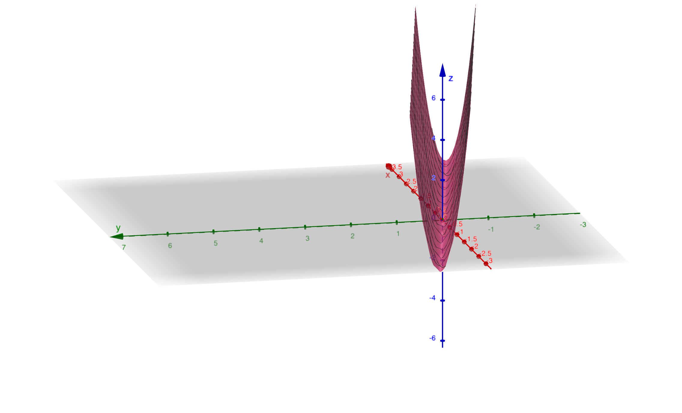
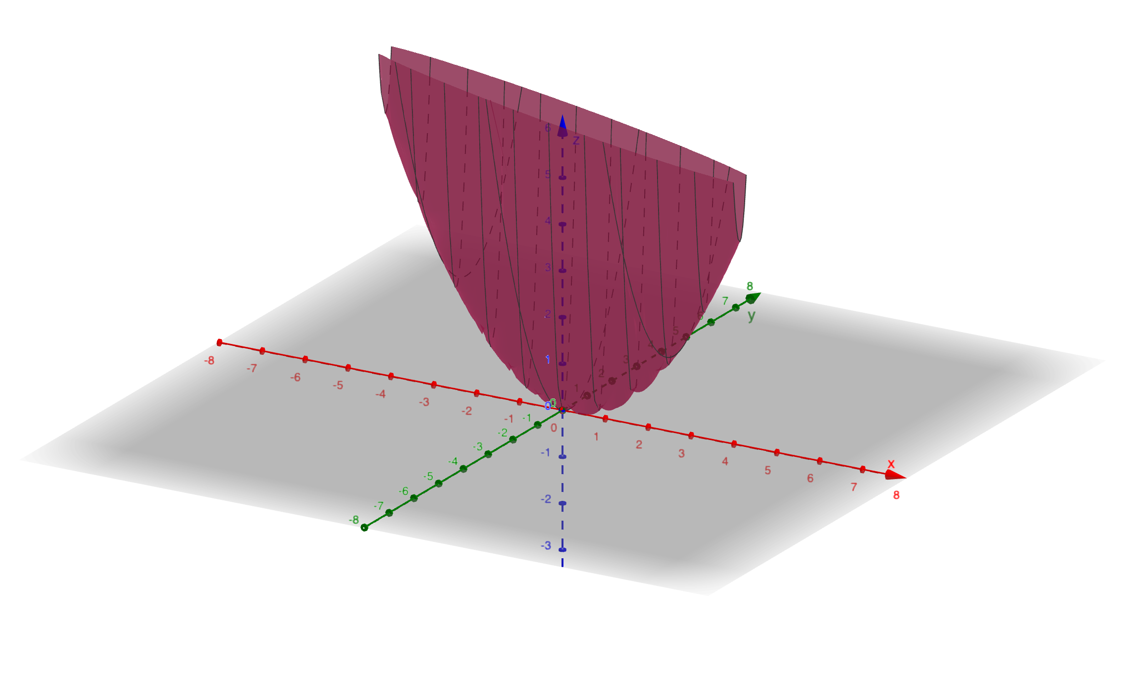
Geometric interpretation: The level curves are ellipses centered at the origin. The function forms a “bowl” with a unique minimum at the origin.
Connection to Elimination
Performing Gaussian elimination: \[ A = \begin{bmatrix}2 & 2 \\ 2 & 20\end{bmatrix} \to U = \begin{bmatrix}2 & 2 \\ 0 & 18\end{bmatrix} \]
Pivots: \([2, 18]\)
Remarkable fact: These pivots appear as the coefficients in the factored form \(f(x, y) = 2(x + y)^2 + 18y^2\). This is no coincidence—the pivots measure the curvature in each direction after eliminating previous variables.
Calculus and the Hessian Matrix
In multivariable calculus, to determine if a critical point is a minimum, we check:
First-order conditions (critical point): \[ \frac{\partial f}{\partial x} = 0, \quad \frac{\partial f}{\partial y} = 0 \]
Second-order conditions (minimum test): \[ \frac{\partial^2 f}{\partial x^2} > 0, \quad \frac{\partial^2 f}{\partial y^2} > 0 \]
More precisely, the Hessian matrix must be positive definite.
The Hessian Matrix
For a function \(f(x, y)\), the Hessian is: \[ H = \begin{bmatrix}f_{xx} & f_{xy} \\ f_{yx} & f_{yy}\end{bmatrix} \]
Key properties: - The Hessian is symmetric because \(f_{xy} = f_{yx}\) (assuming continuous second derivatives) - The Hessian must be positive definite for a minimum - For quadratic forms \(f(x) = x^{\top}Ax\), the Hessian is exactly \(2A\)
Summary Table
| Matrix Type | Geometry | Minima |
|---|---|---|
| Positive Definite | Bowl | Single unique minimum |
| Positive Semidefinite | Bowl with flat line | Infinitely many minima along a line/plane |
| Indefinite | Saddle | No minimum (saddle point) |
3×3 Example
Consider the tridiagonal matrix: \[ A = \begin{bmatrix}2 & -1 & 0 \\ -1 & 2 & -1 \\ 0 & -1 & 2\end{bmatrix} \]
Tests for Positive Definiteness
Leading principal determinants:
- \(\det([2]) = 2 > 0\)
- \(\det\begin{bmatrix}2 & -1 \\ -1 & 2\end{bmatrix} = 4 - 1 = 3 > 0\)
- \(\det(A) = 4 > 0\)
Pivots: \(2, \frac{3}{2}, \frac{4}{3}\) (all positive)
Eigenvalues: \(2 - \sqrt{2}, 2, 2 + \sqrt{2}\) (all positive)
All tests confirm: \(A\) is positive definite.
Quadratic Form
\[ x^{\top}Ax = 2x_1^2 + 2x_2^2 + 2x_3^2 - 2x_1x_2 - 2x_2x_3 \]
This can be factored as: \[ x^{\top}Ax = (x_1 - x_2)^2 + (x_2 - x_3)^2 + x_1^2 + x_3^2 \]
All terms are squares with positive coefficients, confirming positive definiteness.
Geometry: Ellipsoids
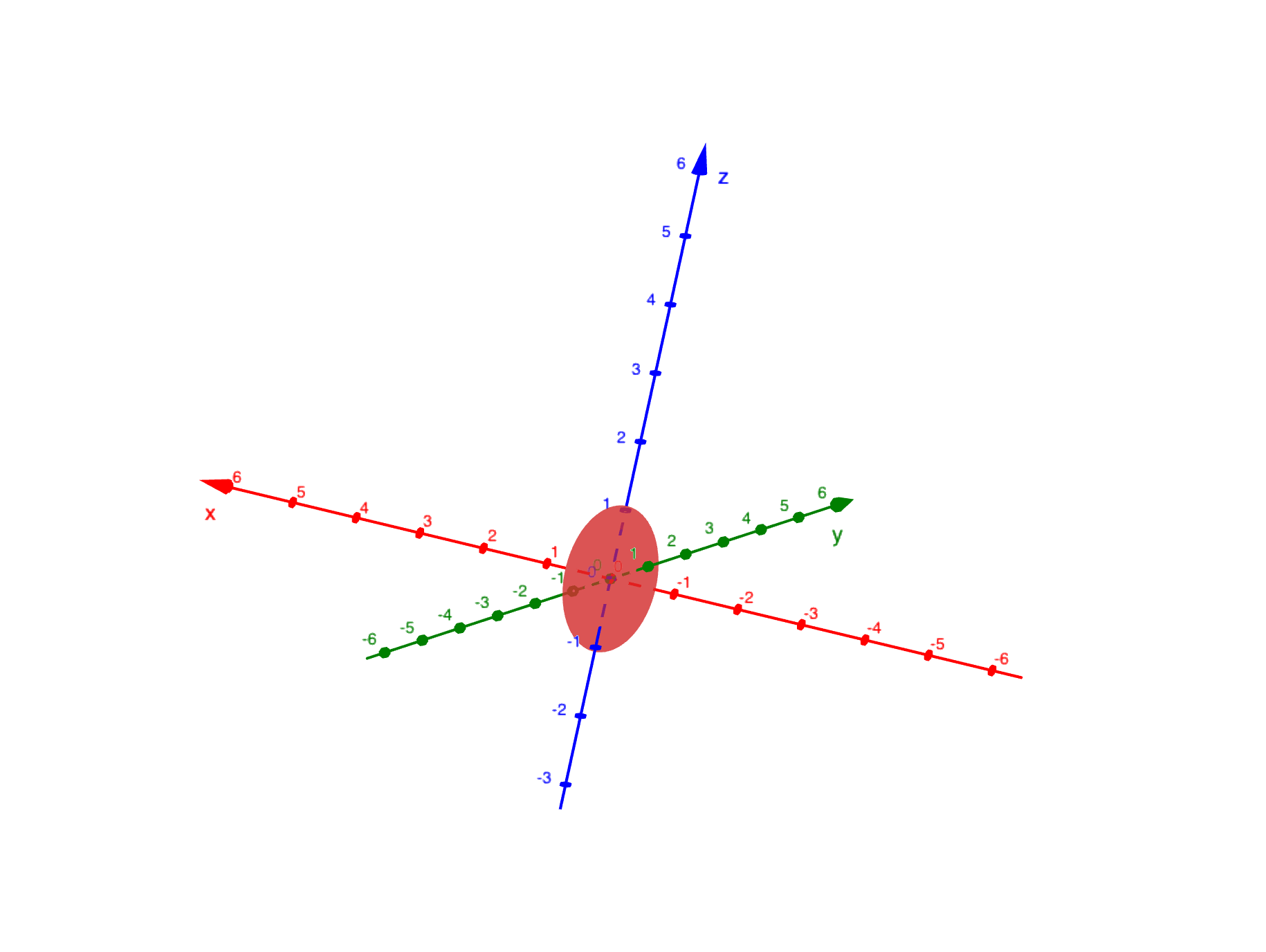
The level surface \(x^{\top}Ax = 1\) is an ellipsoid in 3D space.

Principal Axis Theorem: The spectral decomposition \[ A = Q\Lambda Q^{\top} \]
reveals the geometry: - Eigenvectors (columns of \(Q\)): Principal axes of the ellipsoid - Eigenvalues: Determine the lengths of these axes
For our matrix with eigenvalues \(2 - \sqrt{2}, 2, 2 + \sqrt{2}\): - Major axis: Length proportional to \(\frac{1}{\sqrt{2 - \sqrt{2}}}\) (longest) - Middle axis: Length proportional to \(\frac{1}{\sqrt{2}}\) - Minor axis: Length proportional to \(\frac{1}{\sqrt{2 + \sqrt{2}}}\) (shortest)
Key insight: Larger eigenvalues correspond to directions of greater curvature (tighter curves), resulting in shorter axes on the ellipsoid. Smaller eigenvalues correspond to flatter directions with longer axes.
Summary
This lecture connects positive definite matrices to optimization and geometry:
Four equivalent tests: Energy, eigenvalues, pivots, and determinants all characterize positive definiteness
Semidefinite vs definite: Semidefinite allows zero eigenvalues and has infinitely many minima
Indefinite matrices: Mixed signs in eigenvalues lead to saddle points
Factorization: Completing the square reveals the structure and connects to pivots
Hessian matrix: Second derivatives form a matrix that must be positive definite for a minimum
Geometric interpretation:
- Positive definite → ellipsoid level curves → unique minimum
- Semidefinite → parabolic cylinder → line of minima
- Indefinite → hyperbolic paraboloid → saddle point
Principal Axis Theorem: Eigenvalues and eigenvectors determine the shape and orientation of ellipsoids
Positive definite matrices are fundamental in optimization, machine learning (loss functions), statistics (covariance matrices), and physics (energy functions).