Goodfellow Deep Learning — Chapter 9.1: Convolution Computation
Overview
This section introduces the mathematical foundation of convolutional operations:
- Continuous convolution: Weighted averaging with integral formula
- Discrete convolution: Summation formula for sampled signals
- 2D convolution: Extension to images and spatial data
- Cross-correlation: The operation actually used in most deep learning frameworks
- Concrete example: Step-by-step convolution computation
Convolution is the fundamental operation in convolutional neural networks (CNNs), enabling parameter sharing and translation equivariance.
1. Motivating Example: Noisy Sensor Readings
Problem Setup
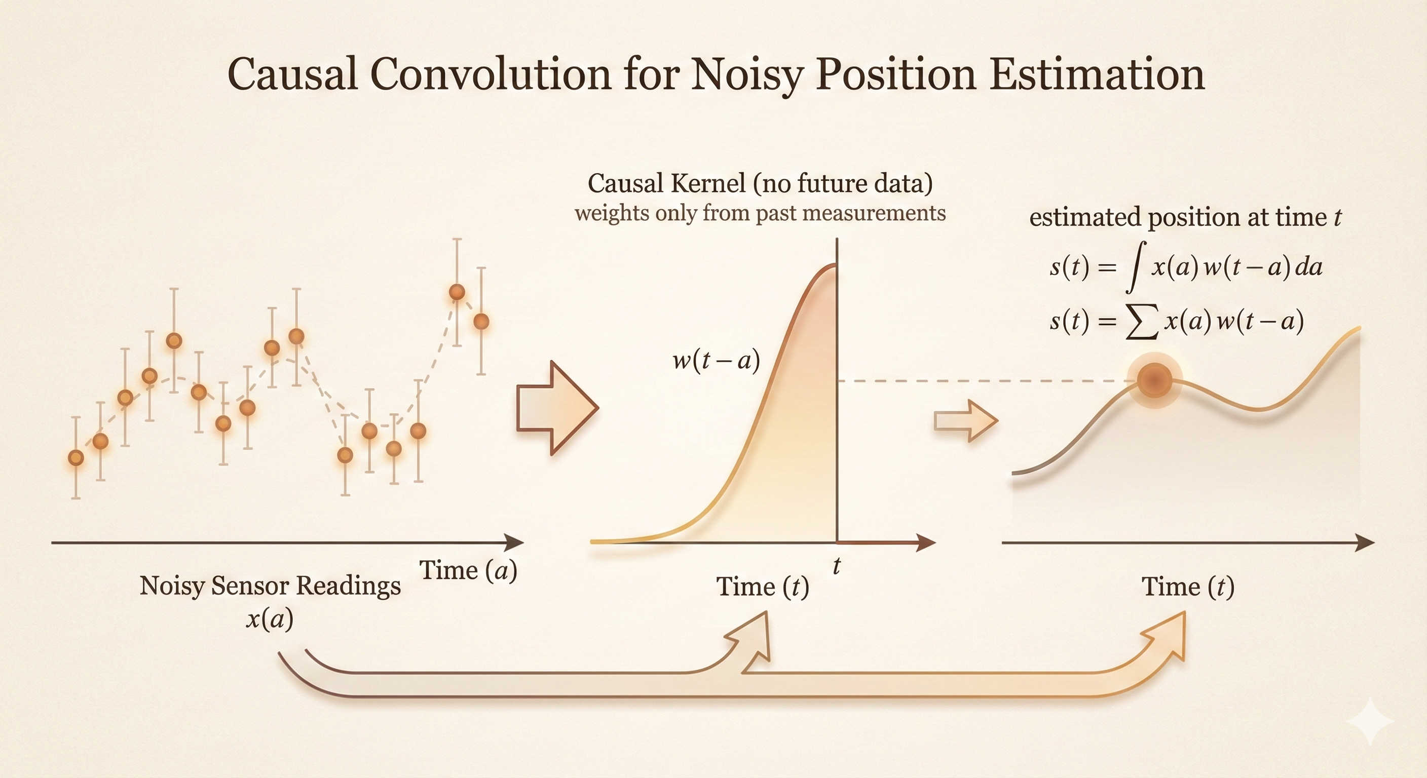
Imagine a spaceship whose exact position at time \(t\) is uncertain because sensor readings include noise.
- \(x(t)\): Raw sensor measurement at time \(t\) (noisy)
- \(s(t)\): Our estimate of the true position at time \(t\)
Instead of trusting a single noisy reading \(x(t)\), we estimate position by taking a weighted average of nearby measurements.
Weighting Function
Define \(w(a)\) as a weighting function where:
\(w(t - a)\) tells us how much the measurement at time \(a\) should contribute to our estimate at time \(t\)
Nearby measurements get higher weight
Distant measurements get lower weight
Typical choice: A Gaussian centered at \(t\):
\[ w(t - a) = \frac{1}{\sqrt{2\pi\sigma^2}} \exp\left(-\frac{(t-a)^2}{2\sigma^2}\right) \]
This gives high weight to measurements close to time \(t\) and low weight to measurements far from \(t\).
2. Continuous Convolution
Definition
The estimated position \(s(t)\) is computed as:
\[ s(t) = \int x(a) w(t - a) \, da \tag{9.1} \]
Interpretation:
For each time \(a\), take the measurement \(x(a)\)
Weight it by \(w(t - a)\) (how relevant time \(a\) is to time \(t\))
Sum (integrate) over all times \(a\)
This operation is called convolution.
Notation
\[ s(t) = (x * w)(t) \tag{9.2} \]
The symbol \(*\) denotes convolution.
 Figure: Physical interpretation of convolution - the output at time \(t\) is computed by sliding the flipped kernel \(w(t-a)\) over the input signal \(x(a)\) and computing the weighted sum.
Properties
Commutativity: \(x * w = w * x\)
Associativity: \((x * w) * z = x * (w * z)\)
Distributivity: \(x * (w + z) = x * w + x * z\)
Smoothing: Convolution with a smooth kernel (like Gaussian) smooths the input signal
Translation equivariance: If input shifts by \(\Delta t\), output shifts by same amount
3. Discrete Convolution
In practice, we work with sampled signals (discrete time points), not continuous functions.
Definition
For discrete signals \(x\) and \(w\), the convolution is:
\[ s(t) = (x * w)(t) = \sum_{a=-\infty}^{\infty} x(a) w(t - a) \tag{9.3} \]
Algorithm:
For each output position \(t\)
For each input position \(a\):
- Take input value \(x(a)\)
- Multiply by weight \(w(t - a)\)
Sum all products
Example
Let \(x = [1, 2, 3, 4]\) and \(w = [0.5, 1, 0.5]\) (centered at index 1).
For \(t = 2\):
\[ s(2) = x(0)w(2) + x(1)w(1) + x(2)w(0) + x(3)w(-1) + \cdots \]
Assuming zero-padding outside the input range:
\[ s(2) = 1 \cdot 0 + 2 \cdot 0.5 + 3 \cdot 1 + 4 \cdot 0.5 = 0 + 1 + 3 + 2 = 6 \]
4. Two-Dimensional Convolution
For images and spatial data, we extend convolution to 2D.
Mathematical Definition (Form 1)
\[ S(i, j) = (I * K)(i, j) = \sum_m \sum_n I(m, n) K(i - m, j - n) \tag{9.4} \]
- \(I(m, n)\): Input image at position \((m, n)\)
- \(K(i - m, j - n)\): Kernel weight for offset \((i - m, j - n)\)
- \(S(i, j)\): Output feature map at position \((i, j)\)
Interpretation: For each output position \((i, j)\), slide the flipped kernel over the input and compute dot product.
Alternative Form (Form 2)
\[ S(i, j) = (I * K)(i, j) = \sum_m \sum_n I(i - m, j - n) K(m, n) \tag{9.5} \]
Interpretation: Equivalently, we can flip the input coordinates instead of the kernel coordinates.
Relationship
Equations (9.4) and (9.5) are equivalent due to commutativity of convolution:
\[ I * K = K * I \]
In practice, we use whichever form is more convenient for implementation.
5. Cross-Correlation
Definition
Most deep learning libraries actually implement cross-correlation, not true convolution:
\[ S(i, j) = (I \star K)(i, j) = \sum_m \sum_n I(i + m, j + n) K(m, n) \tag{9.6} \]
Key difference: The kernel is not flipped (no negative indices \(i - m, j - n\)).
Why the Confusion?
Learned kernels: In CNNs, kernel weights are learned from data, so flipping doesn’t matter—the network will learn the flipped version if needed
Terminology: The operation is still called “convolution” in deep learning, even though it’s technically cross-correlation
Translation equivariance: Both operations preserve translation equivariance, which is the key property for CNNs
Mathematical Relationship
If \(K_{\text{flipped}}(m, n) = K(-m, -n)\), then:
\[ (I * K)(i, j) = (I \star K_{\text{flipped}})(i, j) \]
True convolution with kernel \(K\) equals cross-correlation with flipped kernel \(K_{\text{flipped}}\).
6. Concrete CNN Example
Input Image
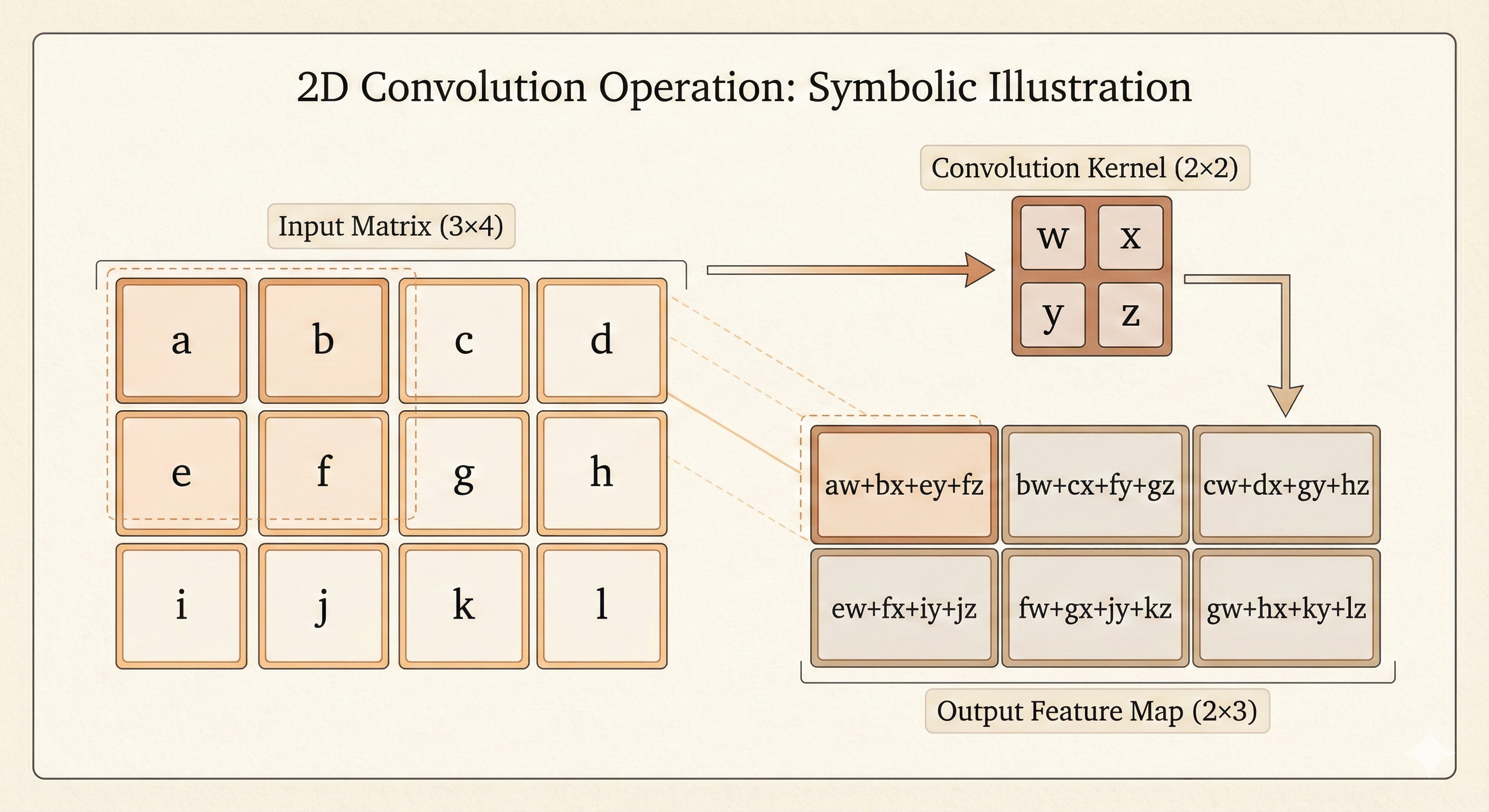
\[ I = \begin{bmatrix} a & b & c & d \\ e & f & g & h \\ i & j & k & l \end{bmatrix} \]
Shape: \(3 \times 4\) (3 rows, 4 columns)
Kernel (Filter)
\[ K = \begin{bmatrix} w & x \\ y & z \end{bmatrix} \]
Shape: \(2 \times 2\)
Computing the Output (Cross-Correlation)
Using equation (9.6), we compute \(S(i, j) = \sum_m \sum_n I(i + m, j + n) K(m, n)\).
Position \((0, 0)\) (top-left):
\[ S(0, 0) = I(0, 0)K(0, 0) + I(0, 1)K(0, 1) + I(1, 0)K(1, 0) + I(1, 1)K(1, 1) \]
\[ = aw + bx + ey + fz \]
Position \((0, 1)\):
\[ S(0, 1) = I(0, 1)K(0, 0) + I(0, 2)K(0, 1) + I(1, 1)K(1, 0) + I(1, 2)K(1, 1) \]
\[ = bw + cx + fy + gz \]
Position \((0, 2)\):
\[ S(0, 2) = I(0, 2)K(0, 0) + I(0, 3)K(0, 1) + I(1, 2)K(1, 0) + I(1, 3)K(1, 1) \]
\[ = cw + dx + gy + hz \]
Position \((1, 0)\):
\[ S(1, 0) = I(1, 0)K(0, 0) + I(1, 1)K(0, 1) + I(2, 0)K(1, 0) + I(2, 1)K(1, 1) \]
\[ = ew + fx + iy + jz \]
Position \((1, 1)\):
\[ S(1, 1) = I(1, 1)K(0, 0) + I(1, 2)K(0, 1) + I(2, 1)K(1, 0) + I(2, 2)K(1, 1) \]
\[ = fw + gx + jy + kz \]
Position \((1, 2)\):
\[ S(1, 2) = I(1, 2)K(0, 0) + I(1, 3)K(0, 1) + I(2, 2)K(1, 0) + I(2, 3)K(1, 1) \]
\[ = gw + hx + ky + lz \]
Output Feature Map
\[ S = \begin{bmatrix} aw + bx + ey + fz & bw + cx + fy + gz & cw + dx + gy + hz \\ ew + fx + iy + jz & fw + gx + jy + kz & gw + hx + ky + lz \end{bmatrix} \]
Shape: \(2 \times 3\)
Output Size Formula
For input size \((H, W)\) and kernel size \((K_H, K_W)\), the output size (with no padding, stride 1) is:
\[ \text{Output height} = H - K_H + 1 = 3 - 2 + 1 = 2 \]
\[ \text{Output width} = W - K_W + 1 = 4 - 2 + 1 = 3 \]
 Figure: Visualization of 2D convolution operation - the kernel slides over the input image, computing dot products at each position to produce the output feature map.
Key Insights
1. Parameter Sharing
The same kernel \(K\) is applied at every spatial location. This dramatically reduces the number of parameters compared to fully connected layers.
Example: For a \(32 \times 32\) image with 64 filters of size \(5 \times 5\):
Convolutional layer: \(5 \times 5 \times 64 = 1{,}600\) parameters
Fully connected layer: \(32 \times 32 \times 32 \times 32 \times 64 = 67{,}108{,}864\) parameters
2. Translation Equivariance
If the input shifts, the output shifts by the same amount:
\[ I'(i, j) = I(i - \Delta i, j - \Delta j) \implies S'(i, j) = S(i - \Delta i, j - \Delta j) \]
This makes CNNs naturally suited for tasks where features can appear anywhere in the image (e.g., object detection).
3. Local Connectivity
Each output unit depends only on a local patch of the input (the receptive field), not the entire input. This:
Reduces computational cost
Captures local spatial structure (edges, corners, textures)
Enables hierarchical feature learning (low-level → mid-level → high-level features)
Summary
| Operation | Formula | Used In |
|---|---|---|
| Continuous Convolution | \(s(t) = \int x(a) w(t - a) \, da\) | Signal processing, theory |
| Discrete Convolution | \(s(t) = \sum_a x(a) w(t - a)\) | Digital signal processing |
| 2D Convolution | \(S(i,j) = \sum_m \sum_n I(m,n) K(i-m, j-n)\) | Image processing (traditional) |
| 2D Cross-Correlation | \(S(i,j) = \sum_m \sum_n I(i+m, j+n) K(m,n)\) | Deep learning (CNNs) |
Key takeaway: Modern deep learning frameworks use cross-correlation (no kernel flipping) but call it “convolution.” Since kernels are learned, the distinction doesn’t affect performance—the network will learn the appropriate kernel regardless of whether it’s flipped or not.