Goodfellow Deep Learning — Deep Learning Book Chapter 7 Prerequisites: Hessian Matrix, Definiteness, and Curvature

Context

My notebook

Before diving into optimization algorithms for deep learning (Chapter 7), we need to understand second-order derivatives in multiple dimensions. The Hessian matrix is the key tool that generalizes the concept of curvature to high-dimensional spaces.

---

Why Second Derivatives Matter

In one dimension, optimizing \(f(x)\) involves:

1. First derivative \(f'(x) = 0\) → Find critical points
   • Why set \(f'(x) = 0\)? At a minimum or maximum, the slope is flat (zero)
   • Think of a hill: at the very top, you stop going up → slope = 0
   • At the bottom of a valley, you stop going down → slope = 0
   • Example: For \(f(x) = x^2\), we have \(f'(x) = 2x\). Setting \(f'(x) = 0\) gives \(x = 0\) (the minimum)
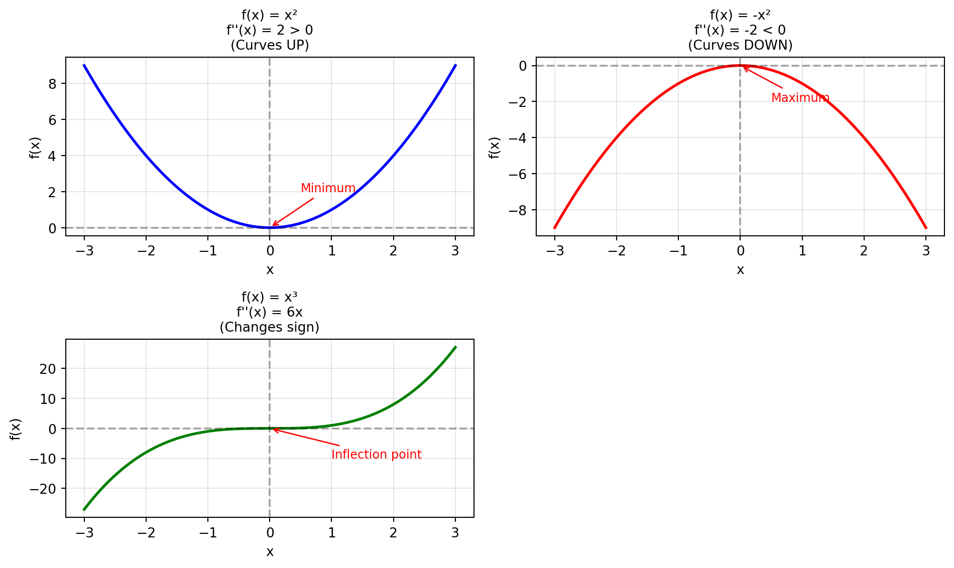
2. Second derivative \(f''(x)\) → Classify the critical point:
   • \(f''(x) > 0\) → Local minimum (curves upward like a bowl)
   • \(f''(x) < 0\) → Local maximum (curves downward like a dome)
   • \(f''(x) = 0\) → Inconclusive (could be an inflection point)
   • Why needed? Not all points where \(f'(x) = 0\) are minima! For \(f(x) = x^3\), we have \(f'(0) = 0\) but it’s neither a min nor max.

The challenge: How do we extend this to functions of many variables \(f(x_1, x_2, \ldots, x_n)\)?

The answer: The Hessian matrix captures all second-order information.

Visualizing Second Derivatives

import numpy as np
import matplotlib.pyplot as plt
from mpl_toolkits.mplot3d import Axes3D

x = np.linspace(-3, 3, 200)

# Three functions with different second derivatives
f1 = x**2           # f''(x) = 2 (positive, curves up)
f2 = -x**2          # f''(x) = -2 (negative, curves down)
f3 = x**3           # f''(x) = 6x (changes sign at x=0)

fig, axes = plt.subplots(2, 2, figsize=(10, 6))

# Function 1: f(x) = x²
axes[0, 0].plot(x, f1, 'b-', linewidth=2)
axes[0, 0].axhline(y=0, color='k', linestyle='--', alpha=0.3)
axes[0, 0].axvline(x=0, color='k', linestyle='--', alpha=0.3)
axes[0, 0].set_title("f(x) = x²\nf''(x) = 2 > 0\n(Curves UP)", fontsize=10)
axes[0, 0].set_xlabel('x')
axes[0, 0].set_ylabel('f(x)')
axes[0, 0].grid(True, alpha=0.3)
axes[0, 0].annotate('Minimum', xy=(0, 0), xytext=(0.5, 2),
                arrowprops=dict(arrowstyle='->', color='red'),
                fontsize=9, color='red')

# Function 2: f(x) = -x²
axes[0, 1].plot(x, f2, 'r-', linewidth=2)
axes[0, 1].axhline(y=0, color='k', linestyle='--', alpha=0.3)
axes[0, 1].axvline(x=0, color='k', linestyle='--', alpha=0.3)
axes[0, 1].set_title("f(x) = -x²\nf''(x) = -2 < 0\n(Curves DOWN)", fontsize=10)
axes[0, 1].set_xlabel('x')
axes[0, 1].set_ylabel('f(x)')
axes[0, 1].grid(True, alpha=0.3)
axes[0, 1].annotate('Maximum', xy=(0, 0), xytext=(0.5, -2),
                arrowprops=dict(arrowstyle='->', color='red'),
                fontsize=9, color='red')

# Function 3: f(x) = x³
axes[1, 0].plot(x, f3, 'g-', linewidth=2)
axes[1, 0].axhline(y=0, color='k', linestyle='--', alpha=0.3)
axes[1, 0].axvline(x=0, color='k', linestyle='--', alpha=0.3)
axes[1, 0].set_title("f(x) = x³\nf''(x) = 6x\n(Changes sign)", fontsize=10)
axes[1, 0].set_xlabel('x')
axes[1, 0].set_ylabel('f(x)')
axes[1, 0].grid(True, alpha=0.3)
axes[1, 0].annotate('Inflection point', xy=(0, 0), xytext=(1, -10),
                arrowprops=dict(arrowstyle='->', color='red'),
                fontsize=9, color='red')

# Hide the unused subplot
axes[1, 1].axis('off')

plt.tight_layout()
plt.show()

Key observations:

Second Derivative	Curvature	Shape	Point Type
\(f''(x) > 0\)	Curves upward	Bowl shape	Potential minimum
\(f''(x) < 0\)	Curves downward	Dome shape	Potential maximum
\(f''(x) = 0\) (at critical point)	Changes sign	Flat at that point	Inflection point

Note on the third example: For \(f(x) = x^3\), we have \(f''(x) = 6x\). At the critical point \(x = 0\), \(f''(0) = 0\), which is inconclusive. The curvature changes sign: negative for \(x < 0\) and positive for \(x > 0\).

---

The Hessian Matrix

Definition

For a scalar function \(f(\mathbf{x}) = f(x_1, x_2, \ldots, x_n)\), the Hessian matrix is the square matrix of all second-order partial derivatives:

\[ H(f) = \begin{bmatrix} \frac{\partial^2 f}{\partial x_1^2} & \frac{\partial^2 f}{\partial x_1 \partial x_2} & \cdots & \frac{\partial^2 f}{\partial x_1 \partial x_n} \\ \frac{\partial^2 f}{\partial x_2 \partial x_1} & \frac{\partial^2 f}{\partial x_2^2} & \cdots & \frac{\partial^2 f}{\partial x_2 \partial x_n} \\ \vdots & \vdots & \ddots & \vdots \\ \frac{\partial^2 f}{\partial x_n \partial x_1} & \frac{\partial^2 f}{\partial x_n \partial x_2} & \cdots & \frac{\partial^2 f}{\partial x_n^2} \end{bmatrix} \]

Key Properties

1. Symmetric: If mixed partial derivatives are continuous, then \(\frac{\partial^2 f}{\partial x_i \partial x_j} = \frac{\partial^2 f}{\partial x_j \partial x_i}\), so \(H = H^T\).

2. Shape: Always \(n \times n\) (determined by number of variables, not terms in the function)

3. Describes curvature in all directions simultaneously

4. Eigenvalue decomposition: Since the Hessian is symmetric, it can be decomposed as \(H = Q\Lambda Q^T\) where \(Q\) contains orthonormal eigenvectors and \(\Lambda\) is a diagonal matrix of eigenvalues

Simple Example

For \(f(x, y) = x^2 + 3y^2\):

Step 1: Compute first derivatives \[ \frac{\partial f}{\partial x} = 2x, \quad \frac{\partial f}{\partial y} = 6y \]

Step 2: Compute second derivatives \[ \frac{\partial^2 f}{\partial x^2} = 2, \quad \frac{\partial^2 f}{\partial y^2} = 6, \quad \frac{\partial^2 f}{\partial x \partial y} = 0 \]

Step 3: Build Hessian \[ H = \begin{bmatrix} 2 & 0 \\ 0 & 6 \end{bmatrix} \]

Interpretation: - Curvature along \(x\)-axis: 2 - Curvature along \(y\)-axis: 6 - No cross-dependency (off-diagonal = 0)

Example with Cross Terms

For \(f(x, y) = x^2 + xy + y^2\):

\[ H = \begin{bmatrix} 2 & 1 \\ 1 & 2 \end{bmatrix} \]

The off-diagonal term (1) indicates that \(x\) and \(y\) are coupled—changing one affects the rate of change of the other.

---

Matrix Definiteness

For a symmetric matrix \(A\), its definiteness is determined by the signs of its eigenvalues.

Type	Eigenvalues	Quadratic Form \(x^T A x\)	Geometric Shape
Positive definite (PD)	all \(> 0\)	\(> 0\) for all \(x \neq 0\)	Bowl (curves upward)
Negative definite (ND)	all \(< 0\)	\(< 0\) for all \(x \neq 0\)	Dome (curves downward)
Indefinite	some \(+\), some \(-\)	depends on direction	Saddle
Positive semi-definite (PSD)	all \(\geq 0\)	\(\geq 0\) for all \(x\)	Flat-bottom bowl
Negative semi-definite (NSD)	all \(\leq 0\)	\(\leq 0\) for all \(x\)	Flat-top dome

Quick Test (2×2 case)

For \(A = \begin{bmatrix} a & b \\ b & c \end{bmatrix}\):

• Positive definite if \(a > 0\) and \(ac - b^2 > 0\)
• Negative definite if \(a < 0\) and \(ac - b^2 > 0\)
• Indefinite if \(ac - b^2 < 0\)

Examples

1. \(\begin{bmatrix} 2 & 0 \\ 0 & 6 \end{bmatrix}\): eigenvalues = [2, 6] → Positive definite

2. \(\begin{bmatrix} -2 & 0 \\ 0 & -3 \end{bmatrix}\): eigenvalues = [-2, -3] → Negative definite

3. \(\begin{bmatrix} 2 & 0 \\ 0 & -2 \end{bmatrix}\): eigenvalues = [2, -2] → Indefinite

4. \(\begin{bmatrix} 2 & 2 \\ 2 & 2 \end{bmatrix}\): eigenvalues = [4, 0] → Positive semi-definite

---

Interpreting Hessian at Critical Points

At a critical point where \(\nabla f = 0\), the Hessian determines the nature of the point:

Hessian Type	Eigenvalues	Surface Shape	Point Type
Positive definite	all positive	Bowl (convex)	Local minimum
Negative definite	all negative	Dome (concave)	Local maximum
Indefinite	mixed signs	Saddle	Neither min nor max
Semi-definite	some zero	Flat in some directions	Inconclusive

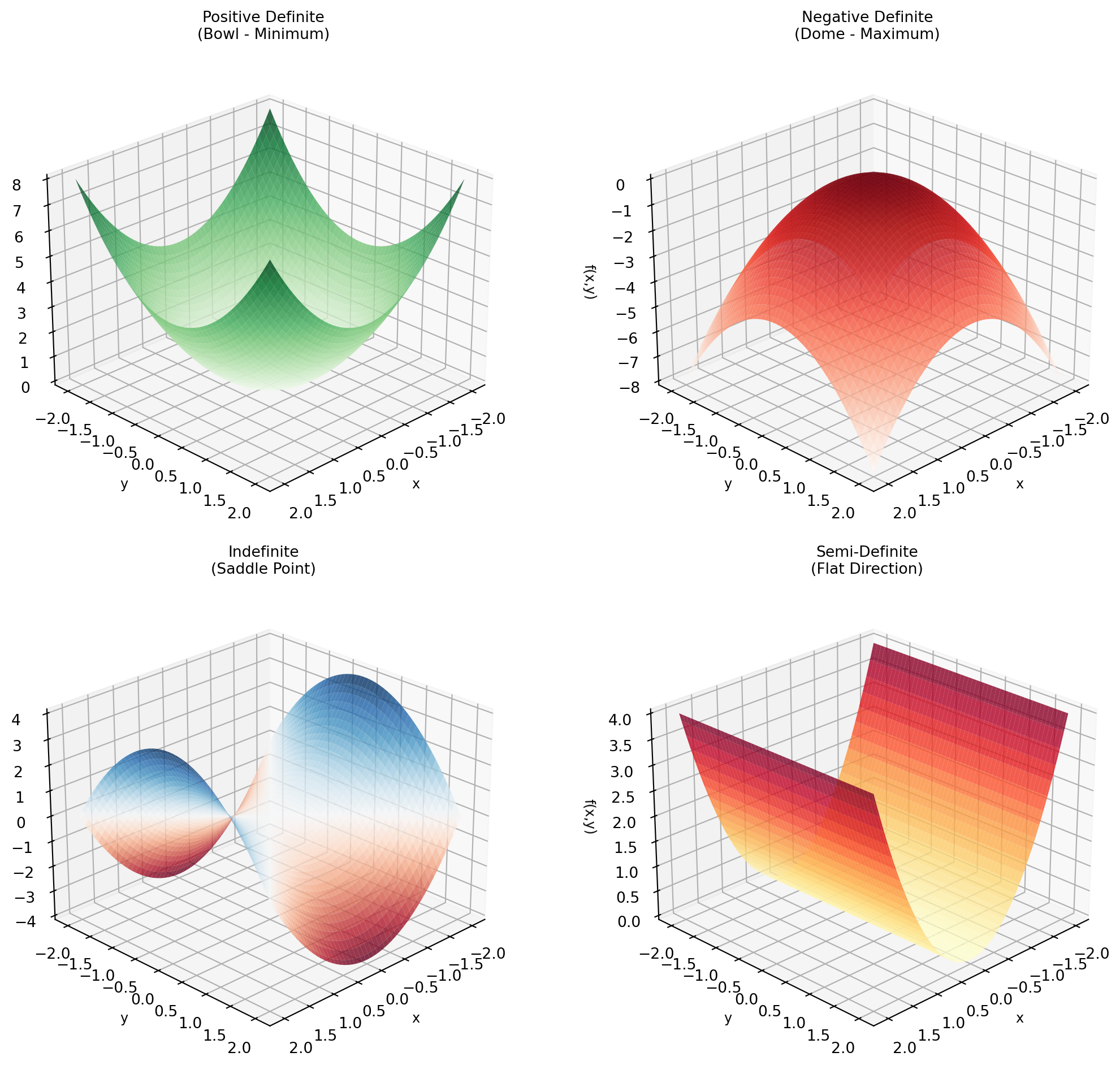
Visualization: Different Surface Types

# Create grid for plotting
x_grid = np.linspace(-2, 2, 100)
y_grid = np.linspace(-2, 2, 100)
X, Y = np.meshgrid(x_grid, y_grid)

# Define different functions with different Hessian types
def positive_definite(x, y):
    """Minimum: f = x² + y²"""
    return x**2 + y**2

def negative_definite(x, y):
    """Maximum: f = -x² - y²"""
    return -x**2 - y**2

def indefinite(x, y):
    """Saddle: f = x² - y²"""
    return x**2 - y**2

def semi_definite(x, y):
    """Flat direction: f = x²"""
    return x**2

# Create 3D surface plots in 2x2 grid
fig = plt.figure(figsize=(12, 10))

functions = [
    (positive_definite, "Positive Definite\n(Bowl - Minimum)", "Greens"),
    (negative_definite, "Negative Definite\n(Dome - Maximum)", "Reds"),
    (indefinite, "Indefinite\n(Saddle Point)", "RdBu"),
    (semi_definite, "Semi-Definite\n(Flat Direction)", "YlOrRd")
]

for idx, (func, title, cmap) in enumerate(functions, 1):
    ax = fig.add_subplot(2, 2, idx, projection='3d')
    Z = func(X, Y)

    surf = ax.plot_surface(X, Y, Z, cmap=cmap, alpha=0.8,
                           linewidth=0, antialiased=True)

    ax.set_xlabel('x', fontsize=9)
    ax.set_ylabel('y', fontsize=9)
    ax.set_zlabel('f(x,y)', fontsize=9)
    ax.set_title(title, fontsize=10)
    ax.view_init(elev=25, azim=45)

plt.tight_layout()
plt.show()

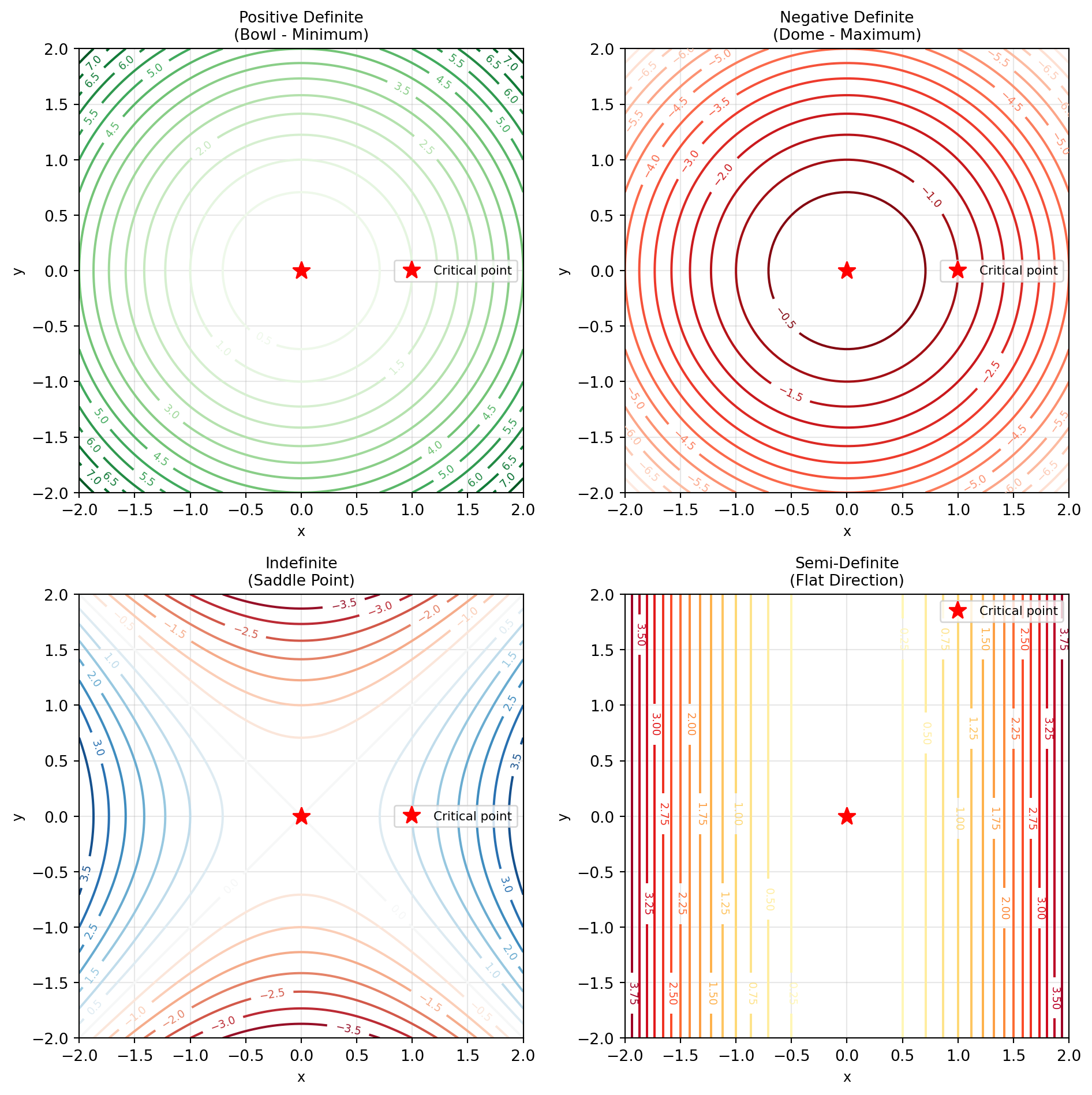
Contour plots for better understanding:

# Contour plots in 2x2 grid
fig, axes = plt.subplots(2, 2, figsize=(10, 10))
axes = axes.flatten()

for idx, (func, title, cmap) in enumerate(functions):
    ax = axes[idx]
    Z = func(X, Y)

    contour = ax.contour(X, Y, Z, levels=15, cmap=cmap)
    ax.clabel(contour, inline=True, fontsize=7)

    # Mark the critical point at origin
    ax.plot(0, 0, 'r*', markersize=12, label='Critical point')

    ax.set_xlabel('x', fontsize=9)
    ax.set_ylabel('y', fontsize=9)
    ax.set_title(title, fontsize=10)
    ax.grid(True, alpha=0.3)
    ax.legend(fontsize=8)
    ax.set_aspect('equal')

plt.tight_layout()
plt.show()