Deep Learning Book 6.1: XOR Problem & ReLU Networks

This recap of Deep Learning Chapter 6.1 shows how ReLU activations let neural networks solve the XOR problem that defeats any linear model.

📓 For a deeper dive with additional exercises and analysis, see the complete notebook on GitHub.

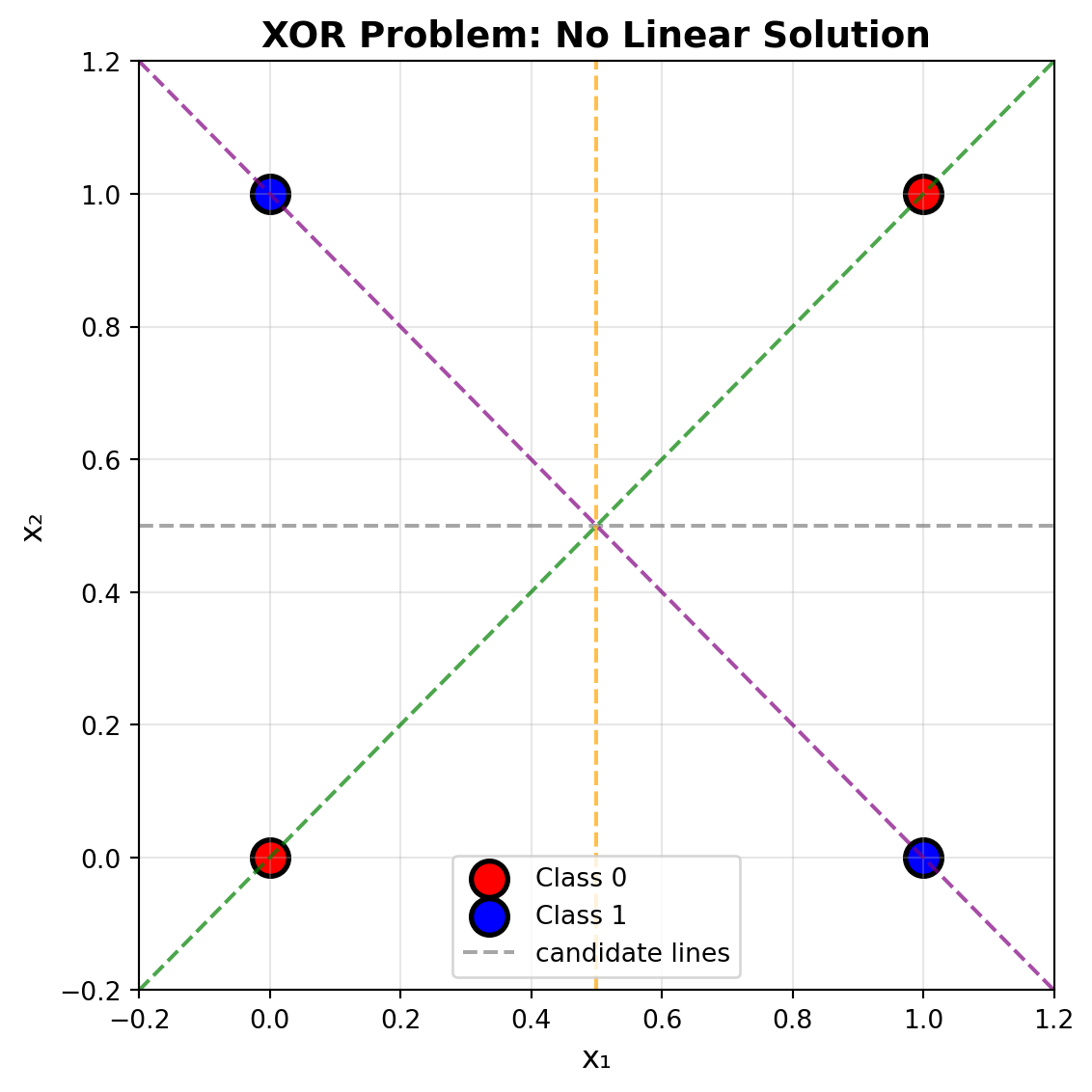
The XOR Problem: A Challenge for Linear Models

XOR (Exclusive OR) returns 1 precisely when the two binary inputs differ:

\[\text{XOR}(x_1, x_2) = \begin{pmatrix}0 & 1\\1 & 0\end{pmatrix}\]

The XOR truth table shows why this is challenging for linear models - the positive class (1) appears at diagonally opposite corners, making it impossible to separate with any single straight line.

import numpy as np
import matplotlib.pyplot as plt
from matplotlib.patches import Rectangle
from sklearn.linear_model import LogisticRegression
from sklearn.neural_network import MLPClassifier
import warnings
warnings.filterwarnings('ignore')

# Define XOR dataset
X = np.array([[0, 0], [0, 1], [1, 0], [1, 1]])
y = np.array([0, 1, 1, 0])

print("XOR Truth Table:")
print("================")
print()
print("┌─────────┬────────┐")
print("│ Input   │ Output │")
print("│ (x₁,x₂) │  XOR   │")
print("├─────────┼────────┤")
for i in range(4):
    input_str = f"({X[i,0]}, {X[i,1]})"
    output_str = f"{y[i]}"
    print(f"│ {input_str:7} │   {output_str:2}   │")
print("└─────────┴────────┘")
print()
print("Notice: XOR = 1 when inputs differ, XOR = 0 when inputs match")

XOR Truth Table:
================

┌─────────┬────────┐
│ Input   │ Output │
│ (x₁,x₂) │  XOR   │
├─────────┼────────┤
│ (0, 0)  │   0    │
│ (0, 1)  │   1    │
│ (1, 0)  │   1    │
│ (1, 1)  │   0    │
└─────────┴────────┘

Notice: XOR = 1 when inputs differ, XOR = 0 when inputs match

Limitation 1: Single Layer Linear Model

A single layer perceptron can only create linear decision boundaries. Let’s see what happens when we try to solve XOR with logistic regression:

# Demonstrate single layer linear model failure
fig, ax = plt.subplots(1, 1, figsize=(6, 6))

colors = ['red', 'blue']

# Plot XOR data
for i in range(2):
    mask = y == i
    ax.scatter(X[mask, 0], X[mask, 1], c=colors[i], s=200, 
               label=f'Class {i}', edgecolors='black', linewidth=2)

# Overlay representative linear separators to illustrate the impossibility
x_line = np.linspace(-0.2, 1.2, 100)
ax.plot(x_line, 0.5 * np.ones_like(x_line), '--', color='gray', alpha=0.7, label='candidate lines')
ax.plot(0.5 * np.ones_like(x_line), x_line, '--', color='orange', alpha=0.7)
ax.plot(x_line, x_line, '--', color='green', alpha=0.7)
ax.plot(x_line, 1 - x_line, '--', color='purple', alpha=0.7)

ax.set_xlim(-0.2, 1.2)
ax.set_ylim(-0.2, 1.2)
ax.set_xlabel('x₁', fontsize=12)
ax.set_ylabel('x₂', fontsize=12)
ax.set_title('XOR Problem: No Linear Solution', fontsize=14, fontweight='bold')
ax.legend()
ax.grid(True, alpha=0.3)

plt.tight_layout()
plt.show()

# Fit logistic regression just to report its performance
log_reg = LogisticRegression()
log_reg.fit(X, y)
accuracy = log_reg.score(X, y)
print(f'Single layer model accuracy: {accuracy:.1%} - still misclassifies XOR.')

Single layer model accuracy: 50.0% - still misclassifies XOR.

Limitation 2: Multiple Layer Linear Model (Without Activation)

Even stacking multiple linear layers doesn’t help! Multiple linear transformations are mathematically equivalent to a single linear transformation.

Mathematical proof:

\[\text{Layer 1: } h_1 = W_1 x + b_1\] \[\text{Layer 2: } h_2 = W_2 h_1 + b_2 = W_2(W_1 x + b_1) + b_2 = (W_2W_1)x + (W_2b_1 + b_2)\]

Result: Still just \(Wx + b\) (a single linear transformation)

Conclusion: Stacking linear layers without activation functions doesn’t increase the model’s expressive power!

The Solution: ReLU Activation Function

ReLU (Rectified Linear Unit) provides the nonlinearity needed to solve XOR: - ReLU(z) = max(0, z) - Clips negative values to zero, keeping positive values unchanged

Using the hand-crafted network from the next code cell, the forward pass can be written compactly in matrix form:

\[ X = \begin{bmatrix} 0 & 0 \\ 0 & 1 \\ 1 & 0 \\ 1 & 1 \end{bmatrix}, \quad W_1 = \begin{bmatrix} 1 & -1 \\ -1 & 1 \end{bmatrix}, \quad b_1 = \begin{bmatrix} 0 & 0 \end{bmatrix} \]

\[ Z = X W_1^{\top} + b_1 = \begin{bmatrix} 0 & 0 \\ -1 & 1 \\ 1 & -1 \\ 0 & 0 \end{bmatrix}, \qquad H = \text{ReLU}(Z) = \begin{bmatrix} 0 & 0 \\ 0 & 1 \\ 1 & 0 \\ 0 & 0 \end{bmatrix} \]

With output parameters \[ w_2 = \begin{bmatrix} 1 & 1 \end{bmatrix}, \quad b_2 = -0.5 \] the final linear scores are \[ a = H w_2^{\top} + b_2 = \begin{bmatrix} -0.5 \\ 0.5 \\ 0.5 \\ -0.5 \end{bmatrix} \Rightarrow \text{sign}_+(a) = \begin{bmatrix} 0 \\ 1 \\ 1 \\ 0 \end{bmatrix} \]

Here \(\text{sign}_+(a)\) maps non-negative entries to 1 and negative entries to 0. Let’s see how ReLU transforms the XOR problem to make it solvable.

# Hand-crafted network weights and biases that solve XOR
from IPython.display import display, Math

def relu(z):
    return np.maximum(0, z)

W1 = np.array([[1, -1],
               [-1, 1]])
b1 = np.array([0, 0])
w2 = np.array([1, 1])
b2 = -0.5

display(Math(r"\text{Hidden layer: } W_1 = \begin{bmatrix} 1 & -1 \\ -1 & 1 \end{bmatrix}"))
display(Math(r"b_1 = \begin{bmatrix} 0 \\ 0 \end{bmatrix}"))
display(Math(r"\text{Output layer: } w_2 = \begin{bmatrix} 1 & 1 \end{bmatrix}"))
display(Math(r"b_2 = -0.5"))

def forward_pass(X, W1, b1, w2, b2):
    z1 = X @ W1.T + b1
    h1 = relu(z1)
    logits = h1 @ w2 + b2
    return logits, h1, z1

logits, hidden_activations, pre_activations = forward_pass(X, W1, b1, w2, b2)
predictions = (logits >= 0).astype(int)

print("Step-by-step Forward Pass Results:")
print("=" * 80)
print()
print("┌─────────┬──────────────────┬──────────────────┬─────────┬──────────┐")
print("│ Input   │  Before ReLU     │  After ReLU      │  Logit  │   Pred   │")
print("│ (x₁,x₂) │    (z₁, z₂)      │    (h₁, h₂)      │  score  │  class   │")
print("├─────────┼──────────────────┼──────────────────┼─────────┼──────────┤")
for i in range(len(X)):
    x1, x2 = X[i]
    z1_vals = pre_activations[i]
    h1_vals = hidden_activations[i]
    logit = logits[i]
    pred = predictions[i]
    
    input_str = f"({x1:.0f}, {x2:.0f})"
    pre_relu_str = f"({z1_vals[0]:4.1f}, {z1_vals[1]:4.1f})"
    post_relu_str = f"({h1_vals[0]:4.1f}, {h1_vals[1]:4.1f})"
    logit_str = f"{logit:6.2f}"
    pred_str = f"{pred:4d}"
    
    print(f"│ {input_str:7} │ {pre_relu_str:16} │ {post_relu_str:16} │ {logit_str:7} │ {pred_str:8} │")
print("└─────────┴──────────────────┴──────────────────┴─────────┴──────────┘")

accuracy = (predictions == y).mean()
print(f"\nNetwork Accuracy: {accuracy:.0%} ✅")
print("\nKey transformations:")
print("• (-1, 1) → (0, 1) makes XOR(0,1) = 1 separable")
print("• ( 1,-1) → (1, 0) makes XOR(1,0) = 1 separable")

\(\displaystyle \text{Hidden layer: } W_1 = \begin{bmatrix} 1 & -1 \\ -1 & 1 \end{bmatrix}\)

\(\displaystyle b_1 = \begin{bmatrix} 0 \\ 0 \end{bmatrix}\)

\(\displaystyle \text{Output layer: } w_2 = \begin{bmatrix} 1 & 1 \end{bmatrix}\)

\(\displaystyle b_2 = -0.5\)

Step-by-step Forward Pass Results:
================================================================================

┌─────────┬──────────────────┬──────────────────┬─────────┬──────────┐
│ Input   │  Before ReLU     │  After ReLU      │  Logit  │   Pred   │
│ (x₁,x₂) │    (z₁, z₂)      │    (h₁, h₂)      │  score  │  class   │
├─────────┼──────────────────┼──────────────────┼─────────┼──────────┤
│ (0, 0)  │ ( 0.0,  0.0)     │ ( 0.0,  0.0)     │  -0.50  │    0     │
│ (0, 1)  │ (-1.0,  1.0)     │ ( 0.0,  1.0)     │   0.50  │    1     │
│ (1, 0)  │ ( 1.0, -1.0)     │ ( 1.0,  0.0)     │   0.50  │    1     │
│ (1, 1)  │ ( 0.0,  0.0)     │ ( 0.0,  0.0)     │  -0.50  │    0     │
└─────────┴──────────────────┴──────────────────┴─────────┴──────────┘

Network Accuracy: 100% ✅

Key transformations:
• (-1, 1) → (0, 1) makes XOR(0,1) = 1 separable
• ( 1,-1) → (1, 0) makes XOR(1,0) = 1 separable

Transformation Table: How ReLU Solves XOR

Let’s trace through exactly what happens to each input:

# Create detailed transformation table
print("Complete Transformation Table:")
print("=============================")
print()
print("Input   | Pre-ReLU  | Post-ReLU | Logit | Prediction | Target | Correct?")
print("(x₁,x₂) | (z₁, z₂)  | (h₁, h₂)  | score | class      | y      |")
print("--------|-----------|-----------|-------|------------|--------|----------")

for i in range(4):
    input_str = f"({X[i,0]},{X[i,1]})"
    pre_relu_str = f"({pre_activations[i,0]:2.0f},{pre_activations[i,1]:2.0f})"
    post_relu_str = f"({hidden_activations[i,0]:.0f},{hidden_activations[i,1]:.0f})"
    logit_str = f"{logits[i]:.2f}"
    pred_str = f"{predictions[i]}"
    target_str = f"{y[i]}"
    correct_str = "✓" if predictions[i] == y[i] else "✗"

    print(f"{input_str:7} | {pre_relu_str:9} | {post_relu_str:9} | {logit_str:5} | {pred_str:10} | {target_str:6} | {correct_str}")

print()
print("Key Insight: ReLU transforms (-1,1) → (0,1) and (1,-1) → (1,0)")
print("This makes the XOR classes linearly separable in the hidden space!")

Complete Transformation Table:
=============================

Input   | Pre-ReLU  | Post-ReLU | Logit | Prediction | Target | Correct?
(x₁,x₂) | (z₁, z₂)  | (h₁, h₂)  | score | class      | y      |
--------|-----------|-----------|-------|------------|--------|----------
(0,0)   | ( 0, 0)   | (0,0)     | -0.50 | 0          | 0      | ✓
(0,1)   | (-1, 1)   | (0,1)     | 0.50  | 1          | 1      | ✓
(1,0)   | ( 1,-1)   | (1,0)     | 0.50  | 1          | 1      | ✓
(1,1)   | ( 0, 0)   | (0,0)     | -0.50 | 0          | 0      | ✓

Key Insight: ReLU transforms (-1,1) → (0,1) and (1,-1) → (1,0)
This makes the XOR classes linearly separable in the hidden space!

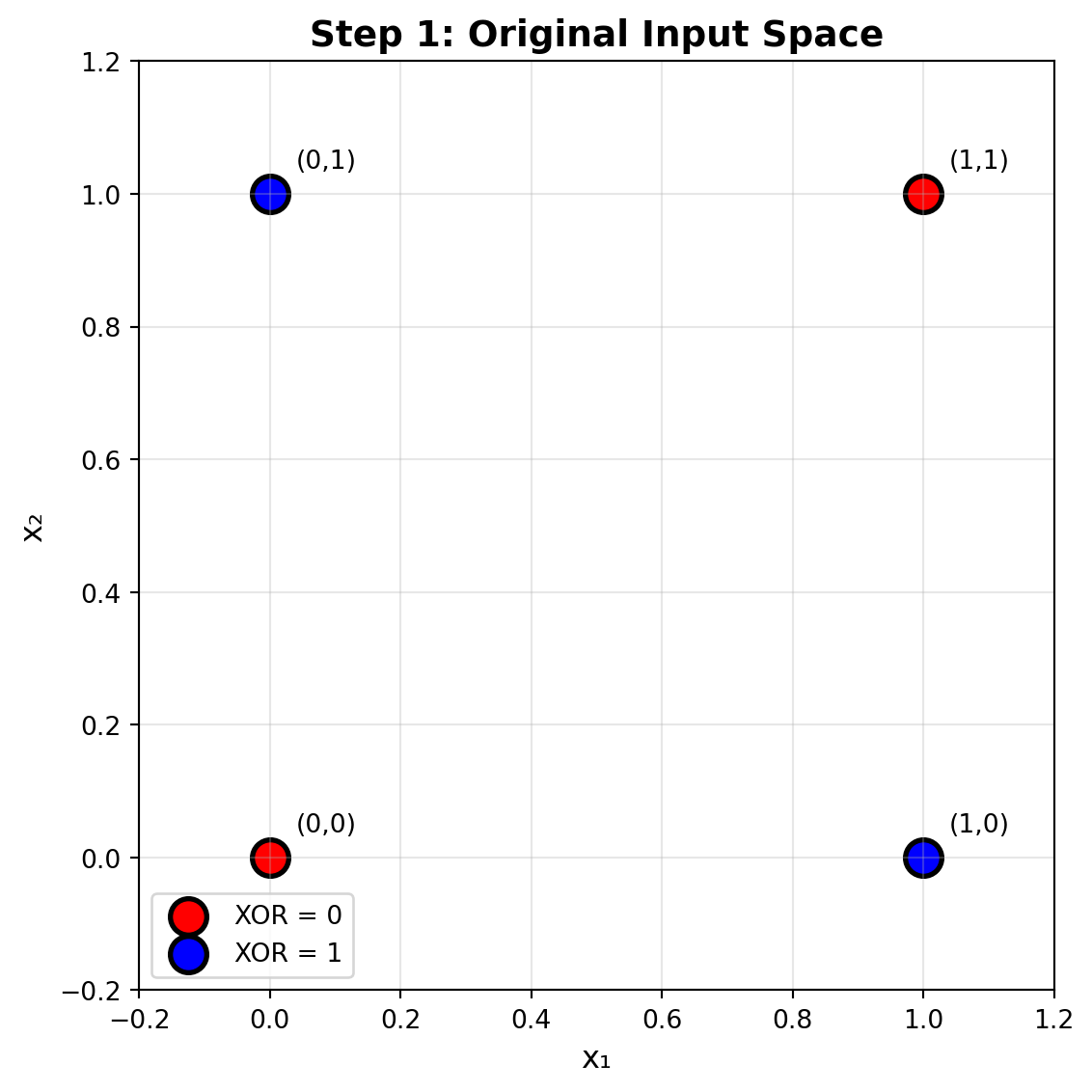
Step 1: Original Input Space

The XOR problem in its raw form - notice how no single line can separate the classes:

# Step 1 visualization: Original Input Space
fig, ax = plt.subplots(1, 1, figsize=(6, 6))

for i in range(2):
    mask = y == i
    ax.scatter(X[mask, 0], X[mask, 1], c=colors[i], s=200, 
               label=f'XOR = {i}', edgecolors='black', linewidth=2)

# Annotate each point
for i in range(4):
    ax.annotate(f'({X[i,0]},{X[i,1]})', X[i], xytext=(10, 10), 
                textcoords='offset points', fontsize=10)

ax.set_xlim(-0.2, 1.2)
ax.set_ylim(-0.2, 1.2)
ax.set_xlabel('x₁', fontsize=12)
ax.set_ylabel('x₂', fontsize=12)
ax.set_title('Step 1: Original Input Space', fontsize=14, fontweight='bold')
ax.legend()
ax.grid(True, alpha=0.3)

plt.tight_layout()
plt.show()

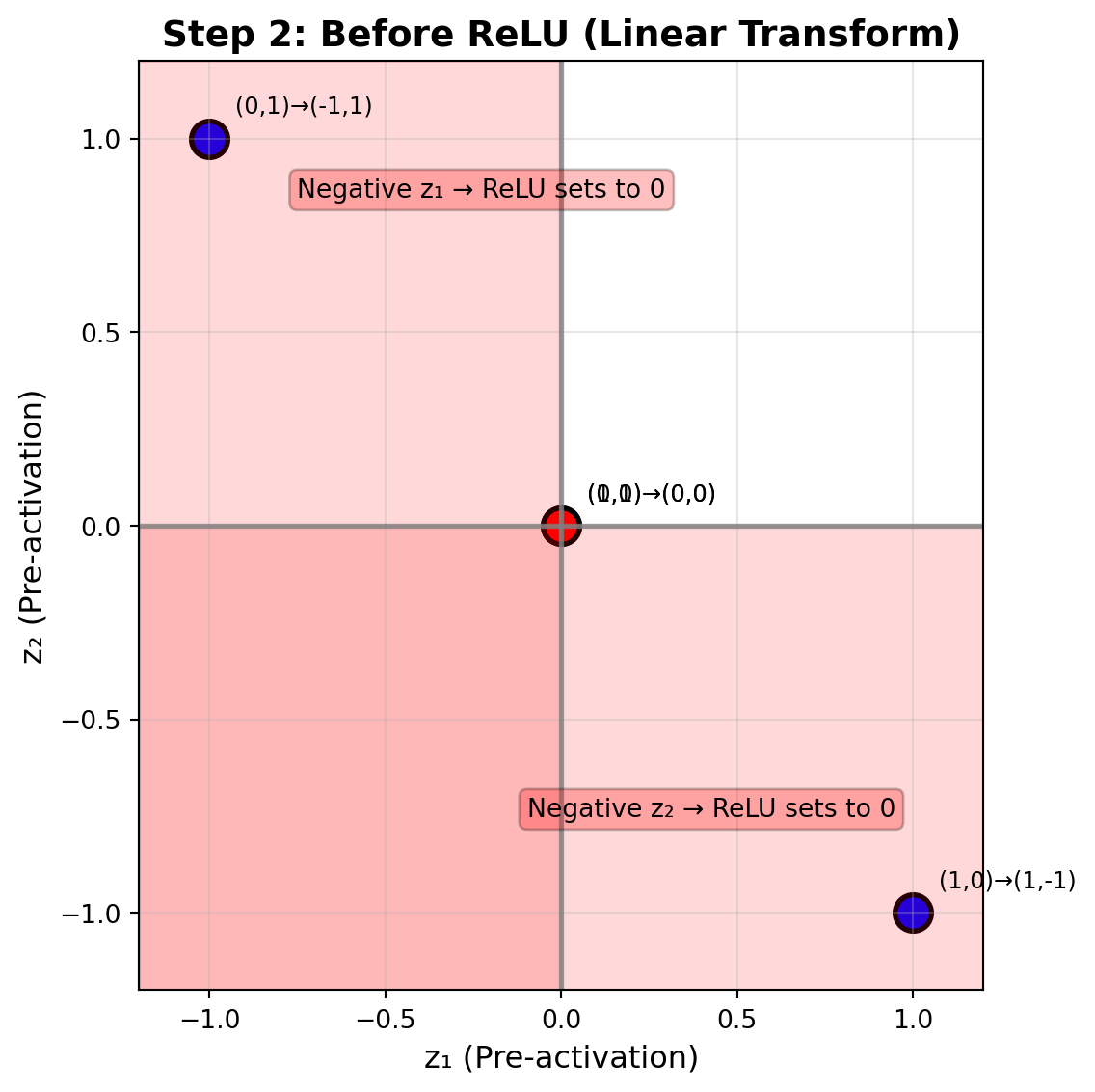
Step 2: Linear Transformation (Before ReLU)

The network applies weights W₁ and biases b₁ to transform the input space:

# Step 2 visualization: Pre-activation space
fig, ax = plt.subplots(1, 1, figsize=(6, 6))

for i in range(4):
    ax.scatter(pre_activations[i, 0], pre_activations[i, 1], 
               c=colors[y[i]], s=200, edgecolors='black', linewidth=2)

# Draw ReLU boundaries
ax.axhline(0, color='gray', linestyle='-', alpha=0.8, linewidth=2)
ax.axvline(0, color='gray', linestyle='-', alpha=0.8, linewidth=2)

# Shade all regions where coordinates turn negative (and thus get clipped by ReLU)
ax.axvspan(-1.2, 0, alpha=0.15, color='red')
ax.axhspan(-1.2, 0, alpha=0.15, color='red')
ax.text(-0.75, 0.85, 'Negative z₁ → ReLU sets to 0', ha='left', fontsize=10,
        bbox=dict(boxstyle='round', facecolor='red', alpha=0.25))
ax.text(0.95, -0.75, 'Negative z₂ → ReLU sets to 0', ha='right', fontsize=10,
        bbox=dict(boxstyle='round', facecolor='red', alpha=0.25))

# Annotate points with input labels
labels = ['(0,0)', '(0,1)', '(1,0)', '(1,1)']
for i, label in enumerate(labels):
    pre_coord = f'({pre_activations[i,0]:.0f},{pre_activations[i,1]:.0f})'
    ax.annotate(f'{label}→{pre_coord}', pre_activations[i], xytext=(10, 10), 
                textcoords='offset points', fontsize=9)

ax.set_xlim(-1.2, 1.2)
ax.set_ylim(-1.2, 1.2)
ax.set_xlabel('z₁ (Pre-activation)', fontsize=12)
ax.set_ylabel('z₂ (Pre-activation)', fontsize=12)
ax.set_title('Step 2: Before ReLU (Linear Transform)', fontsize=14, fontweight='bold')
ax.grid(True, alpha=0.3)

plt.tight_layout()
plt.show()

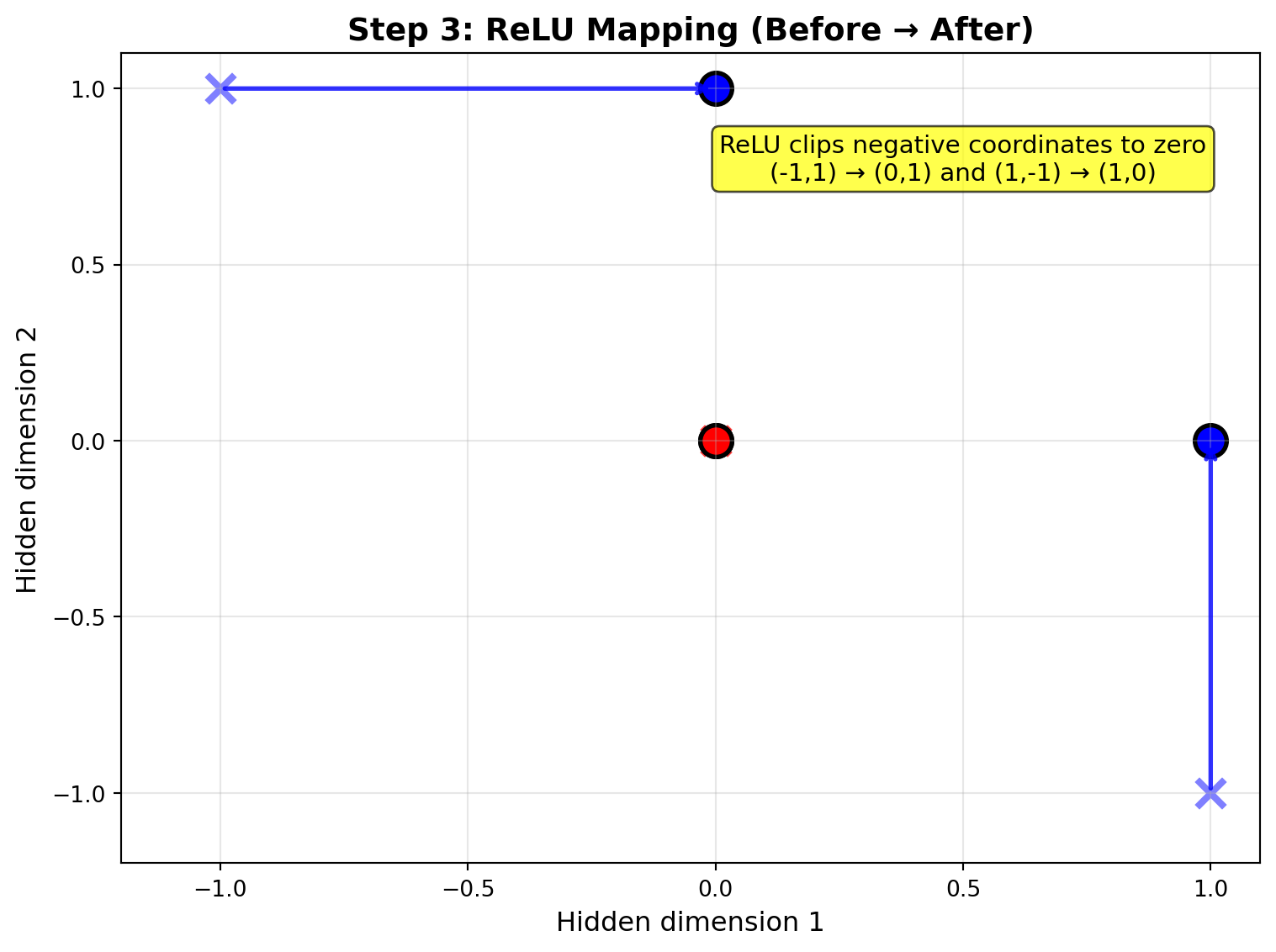
Step 3: ReLU Transformation

ReLU clips negative values to zero, transforming the space to make it linearly separable:

# Step 3 visualization: ReLU transformation with arrows
fig, ax = plt.subplots(1, 1, figsize=(8, 6))

for i in range(4):
    # Pre-ReLU positions (X marks)
    ax.scatter(pre_activations[i, 0], pre_activations[i, 1], 
               marker='x', s=150, c=colors[y[i]], alpha=0.5, linewidth=3)
    # Post-ReLU positions (circles) 
    ax.scatter(hidden_activations[i, 0], hidden_activations[i, 1], 
               marker='o', s=200, c=colors[y[i]], edgecolors='black', linewidth=2)
    
    # Draw transformation arrows
    start = pre_activations[i]
    end = hidden_activations[i]
    if not np.array_equal(start, end):
        ax.annotate('', xy=end, xytext=start,
                    arrowprops=dict(arrowstyle='->', lw=2, color=colors[y[i]], alpha=0.8))


# Add text box explaining the key transformation
ax.text(0.5, 0.8, 'ReLU clips negative coordinates to zero\n(-1,1) → (0,1) and (1,-1) → (1,0)', 
        ha='center', va='center', fontsize=11, 
        bbox=dict(boxstyle='round', facecolor='yellow', alpha=0.7))

ax.set_xlim(-1.2, 1.1)
ax.set_ylim(-1.2, 1.1)
ax.set_xlabel('Hidden dimension 1', fontsize=12)
ax.set_ylabel('Hidden dimension 2', fontsize=12)
ax.set_title('Step 3: ReLU Mapping (Before → After)', fontsize=14, fontweight='bold')
ax.grid(True, alpha=0.3)

plt.tight_layout()
plt.show()

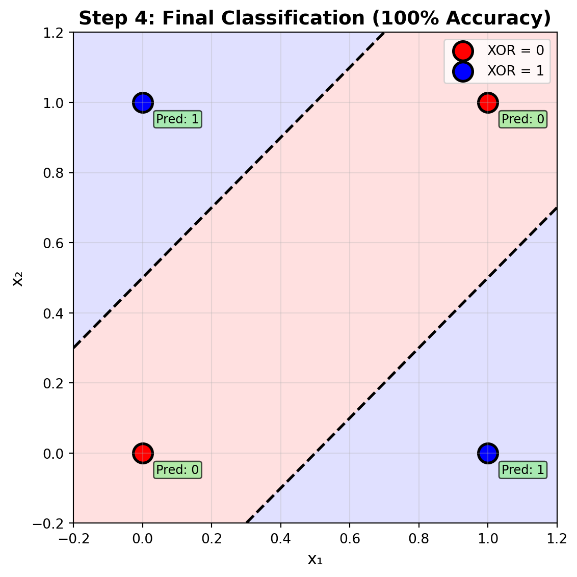
Step 4: Final Classification

With the transformed hidden representation, the network can now perfectly classify XOR:

# Step 4 visualization: Final classification results
fig, ax = plt.subplots(1, 1, figsize=(6, 6))

# Create decision boundary
xx, yy = np.meshgrid(np.linspace(-0.2, 1.2, 100), np.linspace(-0.2, 1.2, 100))
grid_points = np.c_[xx.ravel(), yy.ravel()]
grid_logits, _, _ = forward_pass(grid_points, W1, b1, w2, b2)
grid_preds = (grid_logits >= 0).astype(int).reshape(xx.shape)

ax.contourf(xx, yy, grid_preds, levels=[-0.5, 0.5, 1.5], 
            colors=['#ffcccc', '#ccccff'], alpha=0.6)
ax.contour(xx, yy, grid_logits.reshape(xx.shape), levels=[0], 
           colors='black', linewidths=2, linestyles='--')

for i in range(2):
    mask = y == i
    ax.scatter(X[mask, 0], X[mask, 1], c=colors[i], s=200, 
               label=f'XOR = {i}', edgecolors='black', linewidth=2)

ax.set_xlim(-0.2, 1.2)
ax.set_ylim(-0.2, 1.2)
ax.set_xlabel('x₁', fontsize=12)
ax.set_ylabel('x₂', fontsize=12)
ax.set_title('Step 4: Final Classification (100% Accuracy)', fontsize=14, fontweight='bold')
ax.legend()
ax.grid(True, alpha=0.3)

sample_logits, _, _ = forward_pass(X, W1, b1, w2, b2)
sample_preds = (sample_logits >= 0).astype(int)
for i in range(4):
    pred_text = f'Pred: {sample_preds[i]}'
    ax.annotate(pred_text, X[i], xytext=(10, -15), 
                textcoords='offset points', fontsize=9,
                bbox=dict(boxstyle='round,pad=0.2', facecolor='lightgreen', alpha=0.7))

plt.tight_layout()
plt.show()

Conclusion

The XOR problem demonstrates several fundamental principles in deep learning:

1. Necessity of Nonlinearity: Linear models cannot solve XOR, establishing the critical role of nonlinear activation functions.

2. Universal Approximation: Even simple architectures with sufficient nonlinearity can solve complex classification problems.