Lecture 30: Linear Transformations and Their Matrices
Overview
This lecture explores the fundamental connection between linear transformations and matrices:
- Definition and properties of linear transformations
- Examples of linear and non-linear transformations
- How to represent transformations as matrices using basis
- Constructing the matrix representation from basis vectors
- Examples: projection, rotation, reflection, differentiation
1. Linear Transformations: Definition
A transformation \(T: V \to W\) between vector spaces is linear if it satisfies two properties:
Linearity Rules
- Additivity: \(T(v + w) = T(v) + T(w)\)
- Homogeneity: \(T(cv) = c T(v)\) for any scalar \(c\)
Combined form: \(T(cv + dw) = cT(v) + dT(w)\)
These two properties together ensure that the transformation preserves the vector space structure.
Important Consequence: \(T(0) = 0\)
In any linear transformation, \(T(0)\) must always equal \(0\).
Proof: Using homogeneity with \(c = 0\):
\[ T(0 \cdot v) = 0 \cdot T(v) = 0 \]
Since \(0 \cdot v = 0\) for any vector \(v\), we have \(T(0) = 0\).
Test for non-linearity: If \(T(0) \neq 0\), then \(T\) is immediately not linear.
2. Example 1: Projection (Linear)
Definition
\(T: \mathbb{R}^2 \to \mathbb{R}^2\) where \(T(v)\) projects vector \(v\) onto a line.
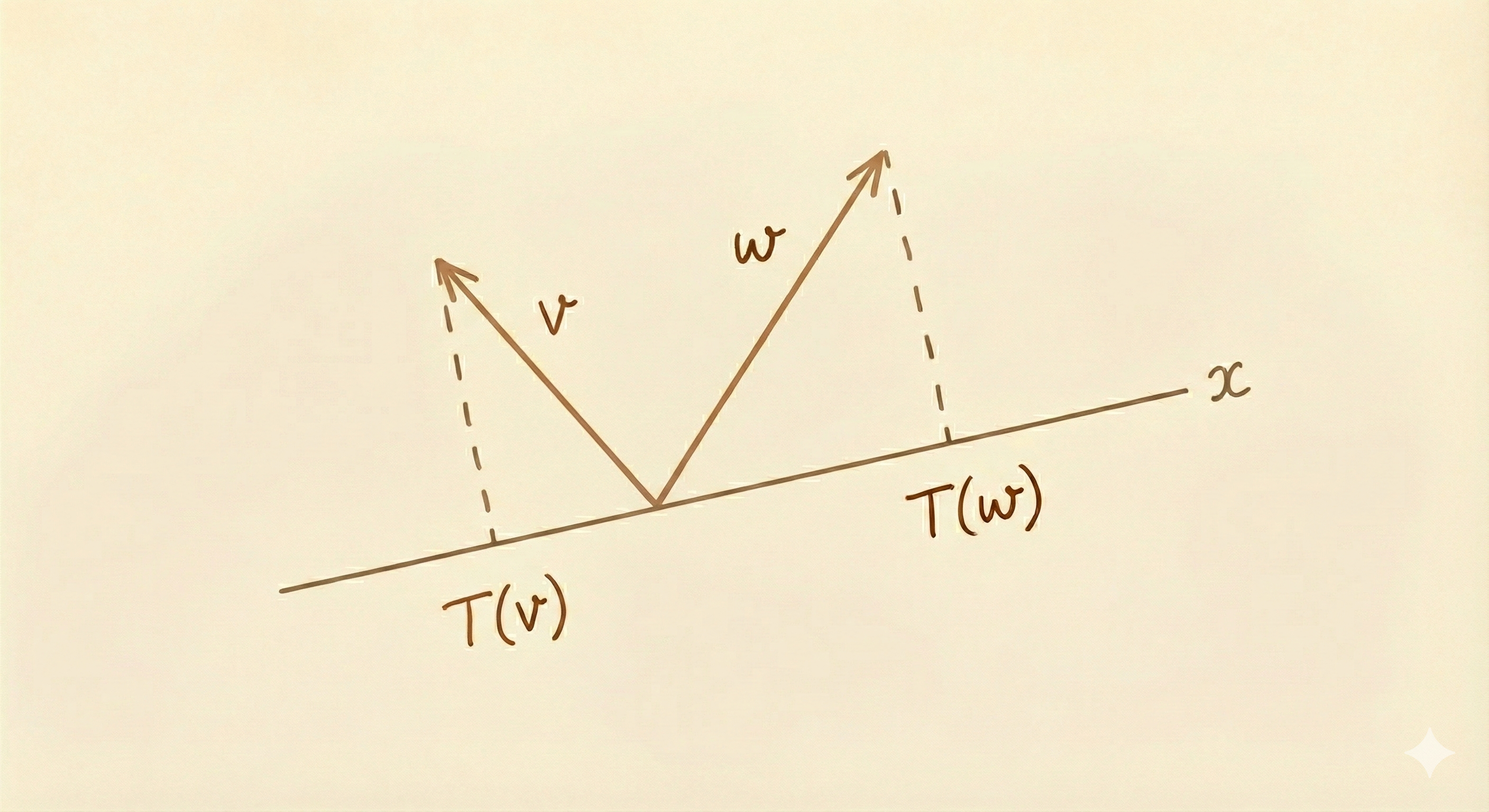 Figure: Projection onto a line - a linear transformation that maps each vector to its closest point on the target line.
Verification of Linearity
Additivity: The projection of \(v + w\) equals the sum of projections:
\[ T(v + w) = T(v) + T(w) \]
Homogeneity: Scaling a vector scales its projection:
\[ T(cv) = c T(v) \]
Both properties are satisfied geometrically: projecting a scaled or summed vector gives the same result as scaling or summing the projections.
3. Example 2: Translation/Shift (NOT Linear)
Definition
\[ T(v) = v + v_0 \]
where \(v_0\) is a fixed non-zero vector.
Why Not Linear?
Check homogeneity with \(c = 2\):
\[ T(2v) = 2v + v_0 \]
But:
\[ 2T(v) = 2(v + v_0) = 2v + 2v_0 \]
Since \(T(2v) \neq 2T(v)\), the transformation is not linear.
Alternative check: \(T(0) = 0 + v_0 = v_0 \neq 0\), which violates the requirement that \(T(0) = 0\).
Key insight: Any transformation that “shifts” the origin is not linear.
4. Example 3: Length/Norm (NOT Linear)
Definition
\[ T(v) = \|v\| \]
(the length of vector \(v\))
Why Not Linear?
Consider \(v \neq 0\) and \(c = -1\):
\[ T(-v) = \|-v\| = \|v\| = T(v) \]
But:
\[ -T(v) = -\|v\| \neq \|v\| \]
Since \(T(-v) \neq -T(v)\), the transformation is not linear.
Intuition: Length is always non-negative, so it cannot satisfy \(T(cv) = cT(v)\) for negative \(c\).
5. Example 4: Rotation (Linear)
Definition
\(T(v)\) rotates vector \(v\) by a fixed angle (e.g., \(45°\)).
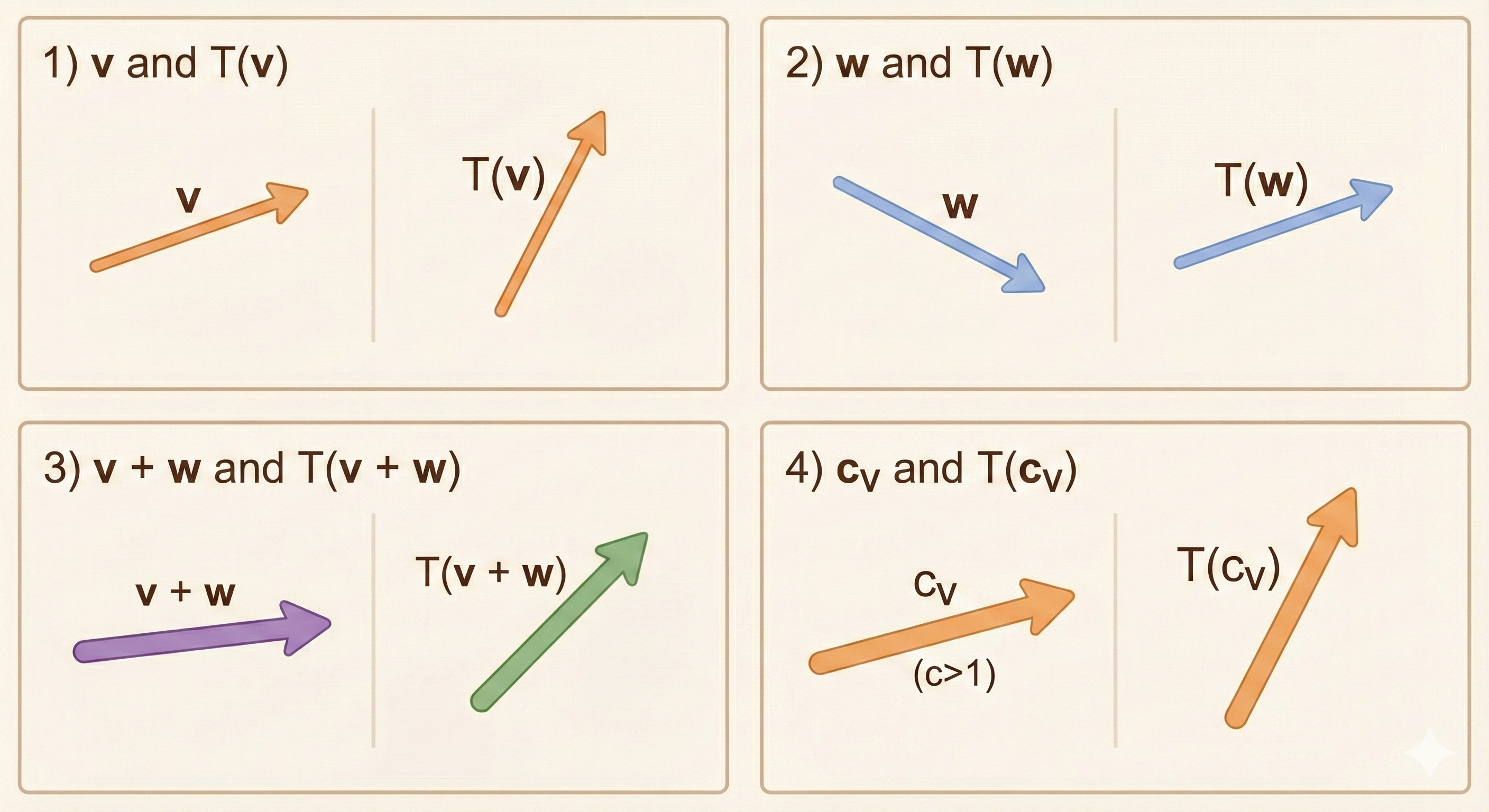 Figure: Rotation by 45° - a linear transformation that preserves lengths and angles between vectors.
Verification of Linearity
Rotation preserves vector addition and scalar multiplication:
- Additivity: Rotating \(v + w\) is the same as adding the rotated vectors
- Homogeneity: Rotating \(cv\) gives \(c\) times the rotated vector
Geometrically, rotation preserves the parallelogram law and scaling.
6. Example 5: Matrix Multiplication (Linear)
Definition
\[ T(v) = Av \]
where \(A\) is a fixed matrix.
Proof of Linearity
Homogeneity:
\[ A(cv) = c(Av) \]
(by properties of matrix multiplication)
Additivity:
\[ A(v + w) = Av + Aw \]
(distributive property)
Therefore, every matrix multiplication defines a linear transformation.
Example: Reflection Across \(x\)-axis
\[ A = \begin{bmatrix} 1 & 0 \\ 0 & -1 \end{bmatrix} \]
This matrix reflects vectors across the \(x\)-axis (flips the \(y\)-coordinate).
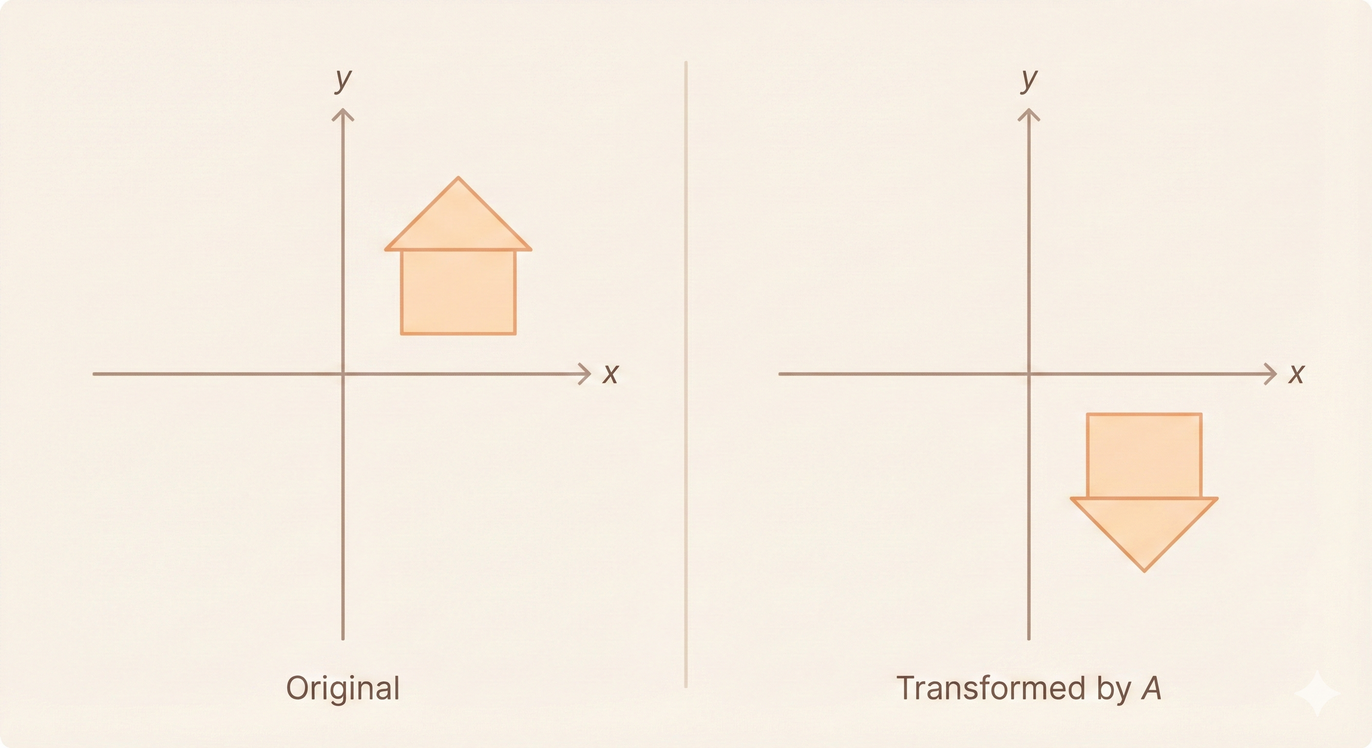 Figure: Reflection across the x-axis - multiplying by this diagonal matrix keeps x unchanged and flips the sign of y.
Action:
\[ \begin{bmatrix} 1 & 0 \\ 0 & -1 \end{bmatrix} \begin{bmatrix} x \\ y \end{bmatrix} = \begin{bmatrix} x \\ -y \end{bmatrix} \]
7. Linear Transformations Between Different Dimensions
Example: \(\mathbb{R}^3 \to \mathbb{R}^2\)
\[ T(v) = Av \]
where \(A\) is a \(2 \times 3\) matrix.
Interpretation: The transformation maps 3D vectors to 2D vectors (a projection from 3D space onto a plane).
Key fact: The dimensions of the input and output spaces determine the size of the matrix.
8. Basis and Coordinates
The Power of Basis
For a linear transformation \(T: \mathbb{R}^n \to \mathbb{R}^m\), if we know the transformation of a basis:
\[ T(v_1), T(v_2), \ldots, T(v_n) \]
then we can compute \(T(v)\) for any vector \(v\).
Why? Every vector \(v\) can be written as a linear combination:
\[ v = c_1 v_1 + c_2 v_2 + \cdots + c_n v_n \]
By linearity:
\[ T(v) = c_1 T(v_1) + c_2 T(v_2) + \cdots + c_n T(v_n) \]
Coordinates
Coordinates come from a choice of basis.
If \(v = c_1 v_1 + \cdots + c_n v_n\), then the coordinate vector of \(v\) in the basis \(\{v_1, \ldots, v_n\}\) is:
\[ [v]_{\{v\}} = \begin{bmatrix} c_1 \\ c_2 \\ \vdots \\ c_n \end{bmatrix} \]
9. Projection in the Cleanest Basis
Choosing the Right Basis
For a projection onto a line in the direction of unit vector \(x\):
Standard basis \(\{e_1, e_2\}\): The matrix is complicated (involves dot products).
Natural basis \(\{x, x^{\perp}\}\) where \(x^{\perp}\) is perpendicular to \(x\):
- \(T(x) = x\) (projection keeps vectors in the direction \(x\) unchanged)
- \(T(x^{\perp}) = 0\) (perpendicular components vanish)
Matrix in this basis:
\[ A_{\{x, x^{\perp}\}} = \begin{bmatrix} 1 & 0 \\ 0 & 0 \end{bmatrix} \]
This is the cleanest possible representation of the projection!
Key insight: The choice of basis dramatically affects how simple the matrix looks.
10. Constructing the Matrix of a Linear Transformation
General Setup
Given: - Input basis: \(v_1, v_2, \ldots, v_n\) (basis for \(\mathbb{R}^n\)) - Output basis: \(w_1, w_2, \ldots, w_m\) (basis for \(\mathbb{R}^m\)) - Linear transformation: \(T: \mathbb{R}^n \to \mathbb{R}^m\)
Goal: Find the \(m \times n\) matrix \(A\) such that \(T\) acts as multiplication by \(A\) in these coordinates.
Constructing the Columns
For each input basis vector \(v_i\), compute \(T(v_i)\) and express it in the output basis:
\[ T(v_i) = a_{1i} w_1 + a_{2i} w_2 + \cdots + a_{mi} w_m \]
The coefficients \([a_{1i}, a_{2i}, \ldots, a_{mi}]^{\top}\) form the \(i\)-th column of \(A\).
Matrix:
\[ A = \begin{bmatrix} | & | & & | \\ [T(v_1)]_{\{w\}} & [T(v_2)]_{\{w\}} & \cdots & [T(v_n)]_{\{w\}} \\ | & | & & | \end{bmatrix} \]
where \([T(v_i)]_{\{w\}}\) denotes the coordinate vector of \(T(v_i)\) in the basis \(\{w_1, \ldots, w_m\}\).
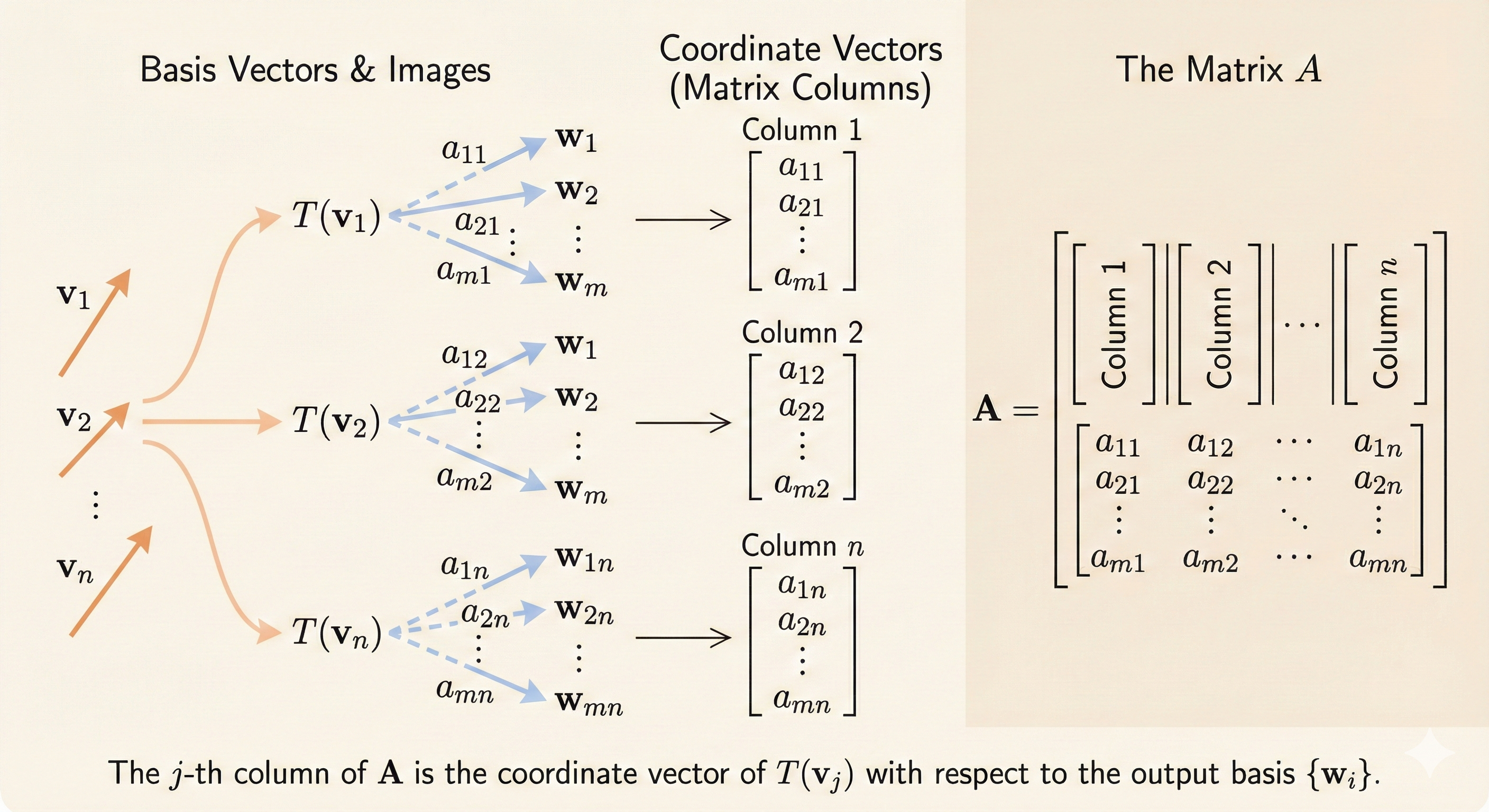 Figure: The matrix of a linear transformation is built column-by-column from the transformed basis vectors, expressed in the output basis coordinates.
11. Example: Differentiation as a Linear Transformation
Setup
Input space: Polynomials of degree \(\leq 2\)
\[ p(x) = c_1 + c_2 x + c_3 x^2 \]
Output space: Polynomials of degree \(\leq 1\)
\[ q(x) = d_1 + d_2 x \]
Transformation: \(T = \frac{d}{dx}\) (differentiation)
Choosing Bases
Input basis: \(\{1, x, x^2\}\)
Output basis: \(\{1, x\}\)
Computing the Matrix
Apply \(T\) to each input basis vector:
- \(T(1) = 0 = 0 \cdot 1 + 0 \cdot x\)
- \(T(x) = 1 = 1 \cdot 1 + 0 \cdot x\)
- \(T(x^2) = 2x = 0 \cdot 1 + 2 \cdot x\)
Matrix:
\[ A = \begin{bmatrix} 0 & 1 & 0 \\ 0 & 0 & 2 \end{bmatrix} \]
Verification
For \(p(x) = c_1 + c_2 x + c_3 x^2\):
\[ A \begin{bmatrix} c_1 \\ c_2 \\ c_3 \end{bmatrix} = \begin{bmatrix} 0 & 1 & 0 \\ 0 & 0 & 2 \end{bmatrix} \begin{bmatrix} c_1 \\ c_2 \\ c_3 \end{bmatrix} = \begin{bmatrix} c_2 \\ 2c_3 \end{bmatrix} \]
This represents:
\[ \frac{d}{dx}(c_1 + c_2 x + c_3 x^2) = c_2 + 2c_3 x \]
Exactly correct!
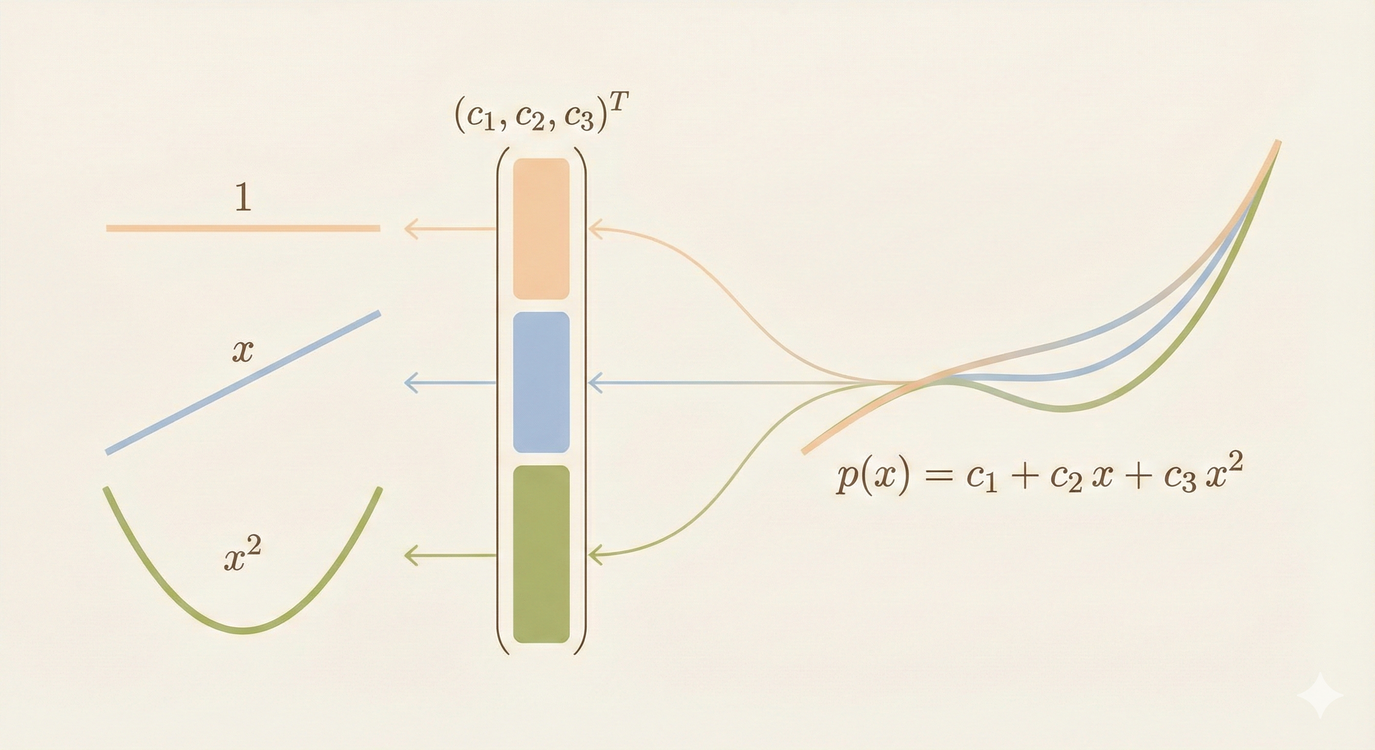 Figure: The derivative operator as a linear transformation - represented by a 2×3 matrix mapping polynomials of degree ≤2 to polynomials of degree ≤1.
Summary
| Concept | Key Idea |
|---|---|
| Linear Transformation | \(T(cv + dw) = cT(v) + dT(w)\) |
| \(T(0) = 0\) | Required for all linear transformations |
| Linear Examples | Projection, rotation, reflection, matrix multiplication, differentiation |
| Non-Linear Examples | Translation/shift, length/norm |
| Matrix Representation | Columns are \(T(v_i)\) expressed in output basis |
| Basis Choice | Right basis makes the matrix simple (e.g., projection is diagonal) |
| Dimensions | \(m \times n\) matrix for \(T: \mathbb{R}^n \to \mathbb{R}^m\) |
Fundamental theorem: Every linear transformation can be represented as matrix multiplication, and every matrix multiplication defines a linear transformation. The choice of basis determines what the matrix looks like.