Chapter 9.2: Motivation for Convolutional Networks

Overview

This section explains the three key motivations for using convolutional neural networks:

• Sparse interactions: Local connectivity reduces parameters and computation
• Parameter sharing: Same kernel used at all positions, enforcing translation invariance
• Translation equivariance: Shifting input shifts output by the same amount

These properties make CNNs particularly well-suited for processing images and other data with spatial structure.

---

1. Sparse Interactions (Local Connectivity)

Dense vs Sparse Connections

Traditional neural networks use dense connections, where every input unit connects to every output unit.

• Each input-output pair has its own unique weight
• Total parameters: O(m · n) where \(m\) = input size, \(n\) = output size
• Computational cost: O(m · n) operations per output

Convolutional neural networks use sparse interactions, because the convolution kernel is much smaller than the input.

• Each output unit only interacts with a small local region of the input (its receptive field)
• Total parameters: O(k · n) where \(k\) = kernel size, and \(k \ll m\)
• Computational cost: O(k · n) operations per output

Benefits of Sparse Connectivity

1. Fewer parameters: Reduces memory requirements and risk of overfitting
2. Less computation: Faster training and inference
3. Meaningful local patterns: CNNs can detect edges, corners, textures
4. Hierarchical features: Deeper layers expand the effective receptive field to model global structure

Key insight: Even though each layer uses sparse connections, units in deeper layers can indirectly connect to a larger region of the input. This allows the network to capture both local and global information efficiently.

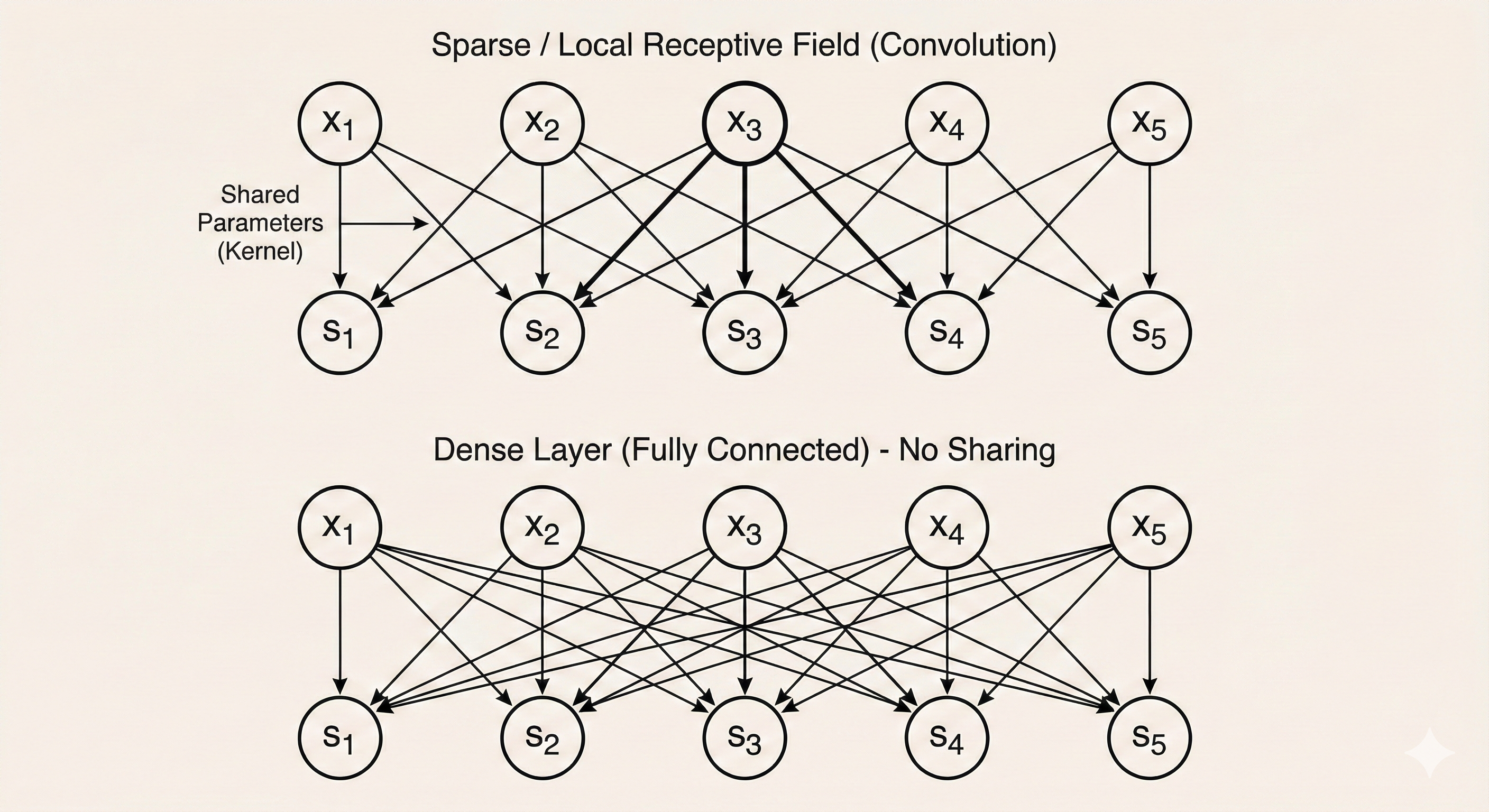Figure: Sparse connectivity - each output (top) connects to only a small local region of the input (bottom), unlike fully connected layers where every output connects to every input.

---

2. Parameter Sharing

Dense Layers: Each Weight Used Once

In a traditional neural network, each weight is used exactly once: - It multiplies one input unit at one position - It is never reused elsewhere in the layer - Different positions require different parameters

Convolutional Layers: Kernel Reuse

In a convolutional neural network, kernel parameters are shared across all spatial positions.

As the kernel slides over the input, the same set of parameters is reused at every location.

Parameter count reduction: - Dense layer: O(m) parameters (one weight per input-output connection) - Convolutional layer: O(k) parameters (only kernel weights)

where \(k \ll m\).

Why Parameter Sharing Works

Parameter sharing enforces a useful inductive bias: patterns detected in one region should also be detectable in other regions.

Examples: - An edge detector that finds vertical edges at the top-left of an image should also detect vertical edges at the bottom-right - A corner detector useful in one part of the image is useful everywhere - The same texture pattern might appear in multiple locations

This assumption is natural for images and many other spatial data, but would not hold for arbitrary data (e.g., different parts of a structured database table might require completely different processing).

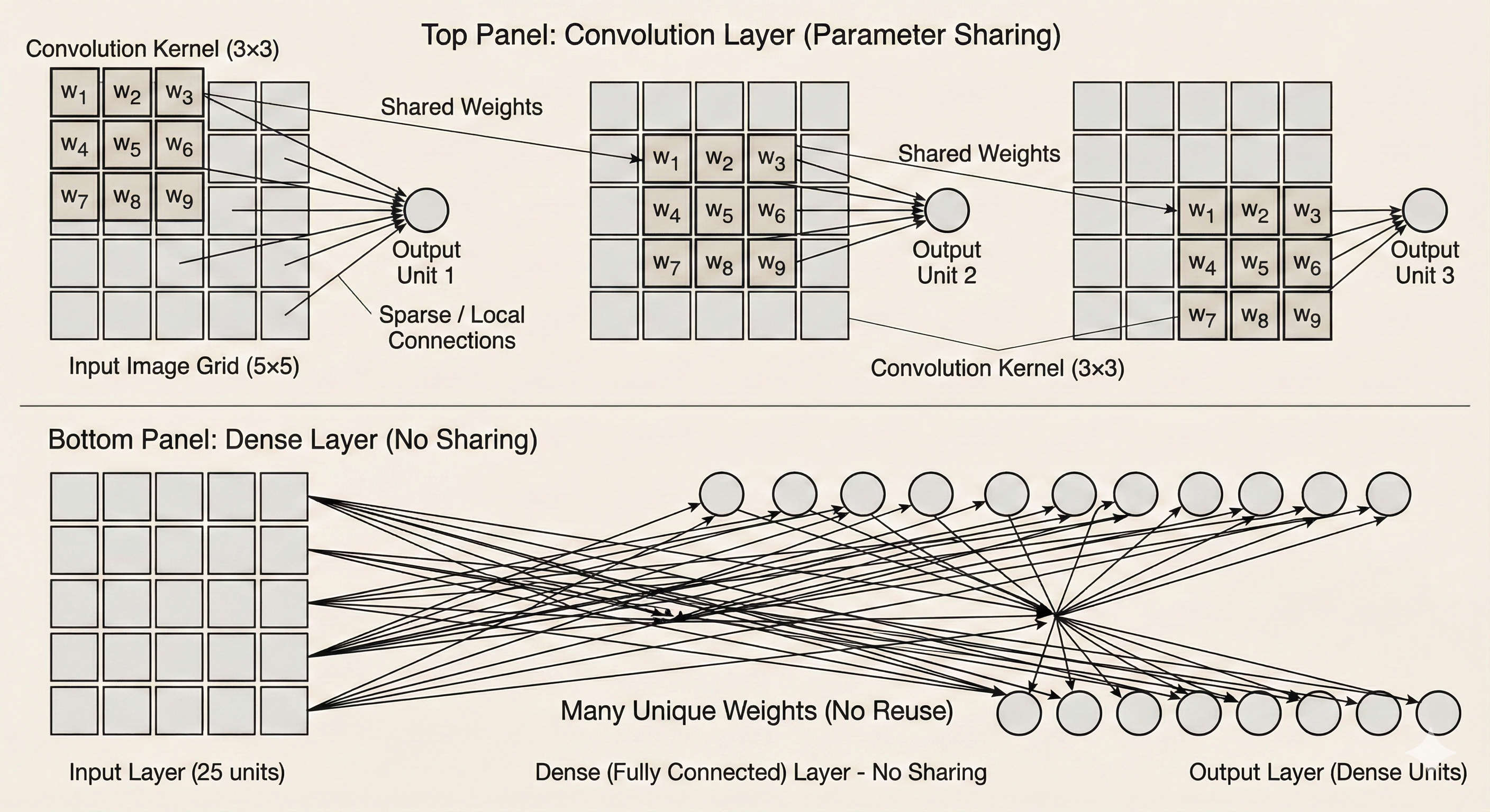Figure: Parameter sharing - the same kernel weights (shown in the same color) are applied at all spatial positions, dramatically reducing the number of parameters compared to fully connected layers.

Receptive Fields Grow with Depth

In CNNs, deeper layers have larger receptive fields than shallow layers.

• Layer 1: Each unit sees a small patch (e.g., 3×3 pixels)
• Layer 2: Each unit sees a larger patch through composition (e.g., 5×5 or 7×7 pixels)
• Layer 3: Even larger effective receptive field (e.g., 11×11 or more)

This hierarchical structure allows the network to build complex features from simple ones: 1. Early layers: Detect simple features (edges, corners, colors) 2. Middle layers: Combine edges into shapes and textures 3. Later layers: Recognize object parts and eventually whole objects

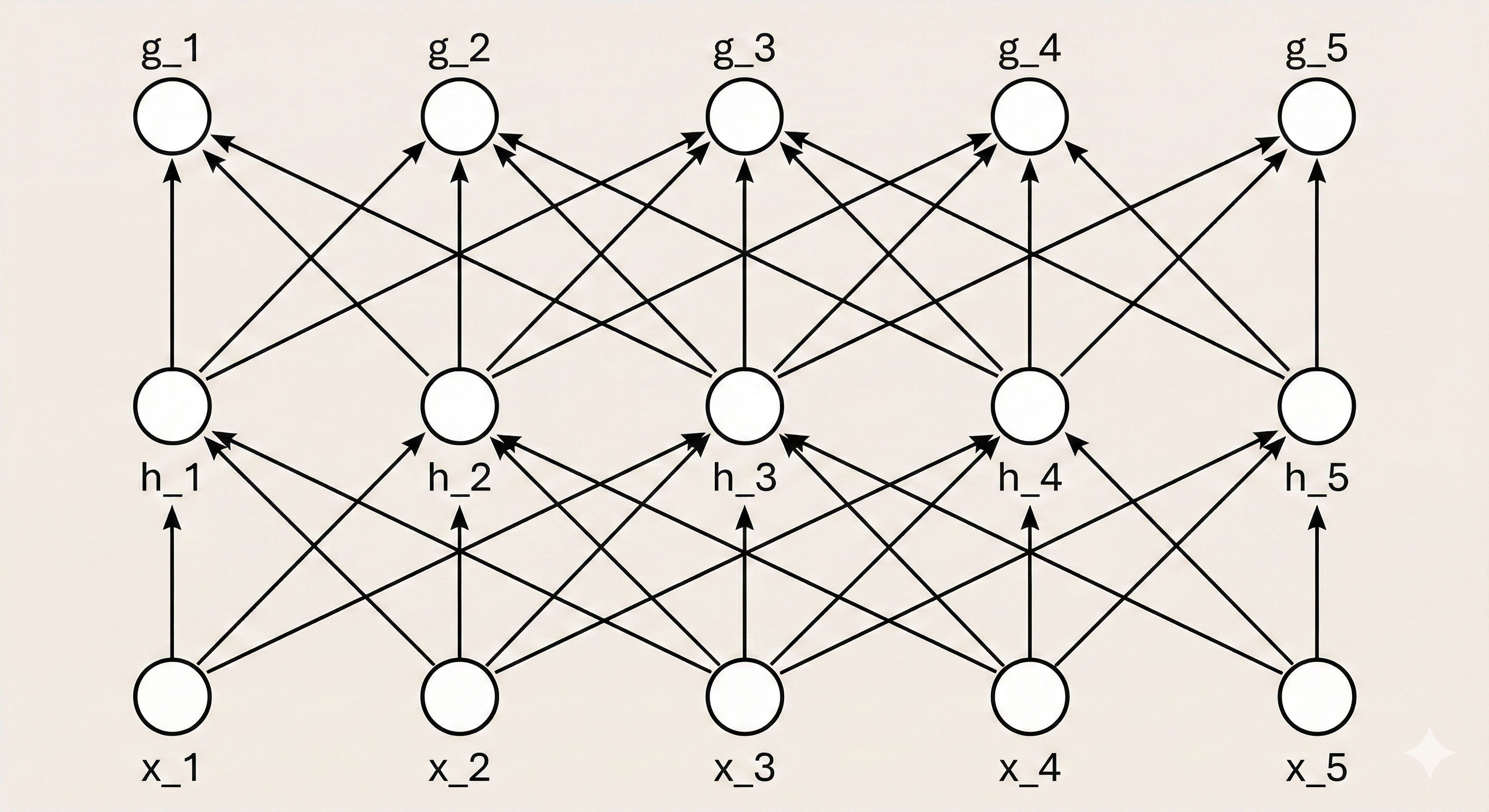Figure: Receptive fields increase with depth - deeper layers can “see” larger regions of the original input through composition of convolutional operations.

---

3. Computational Efficiency

Example: Edge Detection on Images

Consider performing edge detection on a 320 × 280 grayscale image using a 3 × 3 kernel.

Convolutional approach: - Output size: \(319 \times 280\) (with valid padding) - Operations per output: \(3 \times 3 = 9\) multiply-adds - Total operations: \(319 \times 280 \times 3 \approx 2.68 \times 10^5\) operations

Dense matrix multiplication approach: - Unfold each 3×3 patch into a vector - Create a weight matrix of size \((320 \times 280) \times (320 \times 280)\) - Total operations: \(320 \times 280 \times 320 \times 280 \approx 8.03 \times 10^9\) operations

Speedup Factor

\[ \text{Speedup} = \frac{8.03 \times 10^9}{2.68 \times 10^5} \approx 30,000\times \]

Convolution is roughly 30,000 times more efficient than implementing the same operation as a dense matrix multiplication!

This massive speedup comes from: 1. Sparse connectivity: Each output only depends on a local patch 2. Parameter sharing: Same kernel weights used at all positions

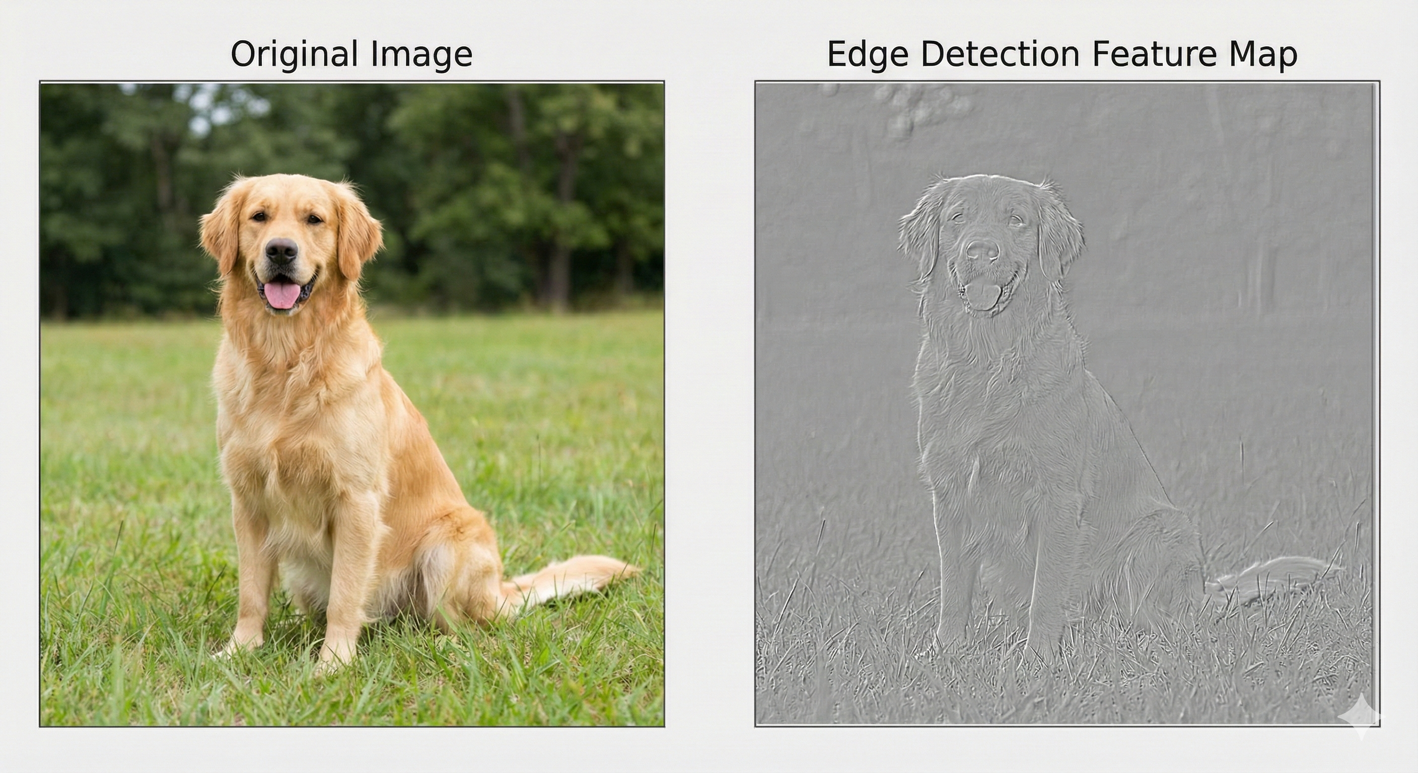Figure: Edge detection example - applying a 3×3 edge detection kernel to an image is vastly more efficient than using a fully connected layer.

Figure: Computational cost comparison - convolutional layers (green) require orders of magnitude fewer operations than dense layers (red) for the same task on images.

---

4. Translation Equivariance

Definition

A convolution is translation-equivariant: if the input is shifted, the output shifts by the same amount while preserving its structure.

Formally, convolution satisfies:

\[ f(g(x)) = g(f(x)) \]

where: - \(f\) is the convolution operation - \(g\) is a spatial translation (shift) - \(x\) is the input

What This Means

Translation equivariance means the network detects the same pattern regardless of its position in the input, producing output feature maps that move consistently with the input.

Example: - If an edge appears at position \((10, 20)\) in the input image - And we shift the image by \((5, 3)\) pixels - The edge detector will fire at position \((10+5, 20+3) = (15, 23)\) in the shifted image

The response is the same, just shifted by the same amount.

Contrast with Translation Invariance

Translation equivariance is different from translation invariance:

• Equivariance: Output shifts when input shifts (CNNs with convolution)
• Invariance: Output stays the same when input shifts (achieved with pooling)

Convolutional layers provide equivariance. Adding pooling layers creates approximate invariance, which is useful for classification tasks where we care about “is there a cat?” but not “where exactly is the cat?”

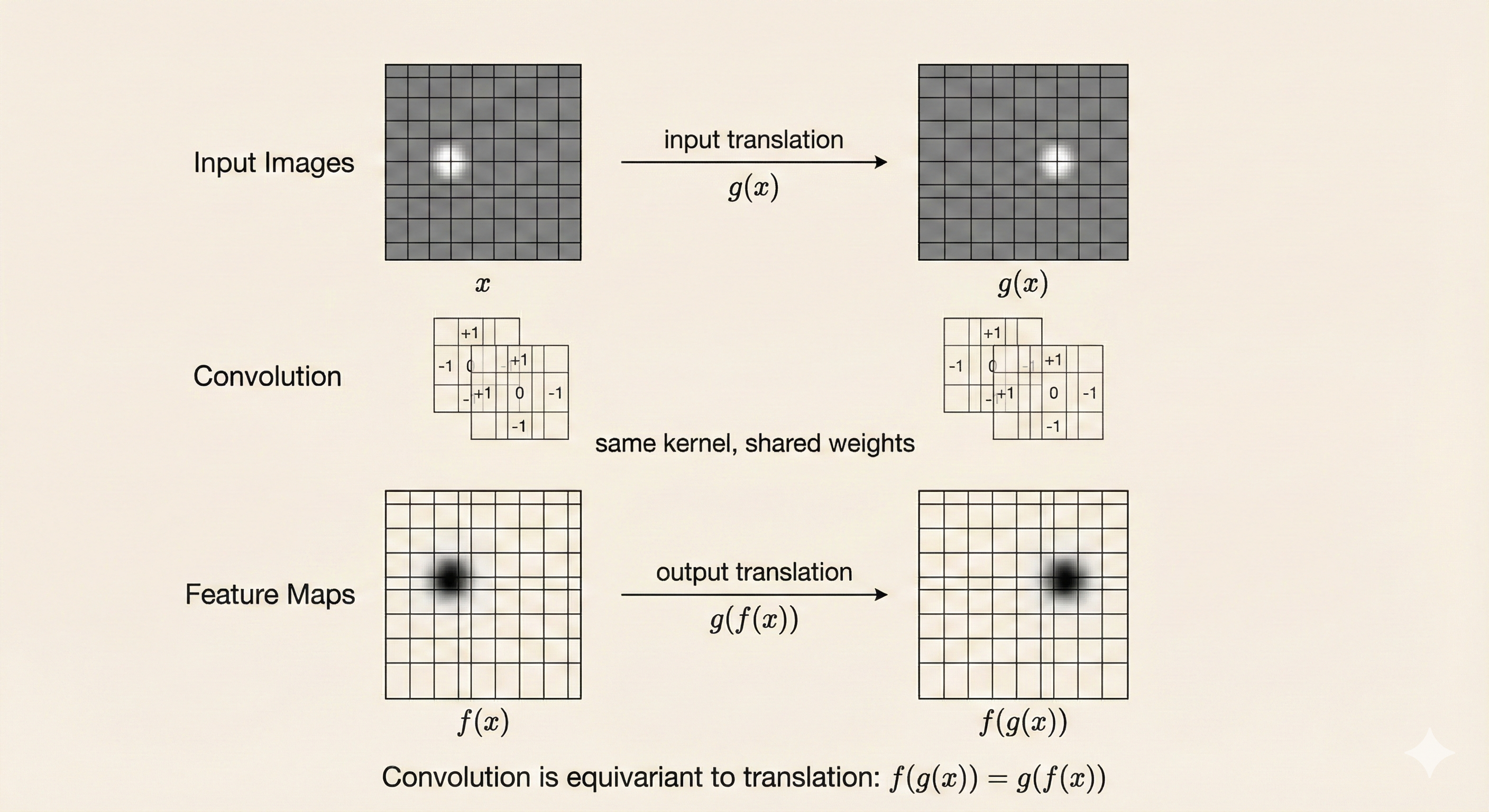Figure: Translation equivariance - when the input is shifted (top), the output feature map shifts by the same amount (bottom), preserving the detection pattern.