Goodfellow Deep Learning — Chapter 9.5: Convolutional Functions
Overview
This section covers the mathematical details and variations of convolutional operations:
- Mathematical vs deep learning convolution (commutativity)
- Multi-channel convolution computation
- Downsampling with stride
- Padding strategies (valid, same, full)
- Local connected layers and tiled convolution
- Gradient computation for backpropagation
- Encoder-decoder architectures
1. Mathematical vs Deep Learning Convolution
Mathematical Convolution (Commutative)
In mathematics, convolution is commutative and invertible:
\[ (f * g)(t) = \sum_\tau f(\tau) \, g(t - \tau) \]
\[ (g * f)(t) = \sum_\tau g(\tau) \, f(t - \tau) \]
Example: When \(\tau = 1\):
\[ f(1)g(t-1) = g(t-1)f(t-(t-1)) = g(t-1)f(1) \]
Key property: \((f * g) = (g * f)\) (commutative)
Deep Learning Convolution (Non-commutative)
In deep learning, we use cross-correlation, which is non-commutative:
\[ (f \star g)(t) = \sum_\tau f(t + \tau) \, g(\tau) \]
\[ (g \star f)(t) = \sum_\tau g(t + \tau) \, f(\tau) \]
Example: When \(\tau = 1\):
\[ f(t+1)g(1) \neq g(t+1)f(1) \]
Key property: \((f \star g) \neq (g \star f)\) (not commutative)
Why this matters: Since kernels are learned, the lack of commutativity doesn’t affect performance—the network will learn the appropriate kernel regardless.
2. Multi-Channel Convolution Computation
Notation
- Input: \(V \in \mathbb{R}^{i \times m \times n}\)
- \(i\): number of input channels
- \(m\): input height
- \(n\): input width
- Kernel: \(K \in \mathbb{R}^{l \times i \times j \times k}\)
- \(l\): number of output channels
- \(i\): number of input channels (must match input)
- \(j\): kernel height
- \(k\): kernel width
- Output: \(Z \in \mathbb{R}^{l \times (m-j+1) \times (n-k+1)}\)
- Assuming stride = 1, no padding
Convolution Formula
\[ Z_{l,x,y} = \sum_{i,j,k} V_{i,x+j-1,y+k-1} \, K_{l,i,j,k} \tag{9.7} \]
Interpretation: - For each output channel \(l\) and spatial position \((x, y)\) - Sum over all input channels \(i\) and all kernel positions \((j, k)\) - Multiply corresponding input and kernel values
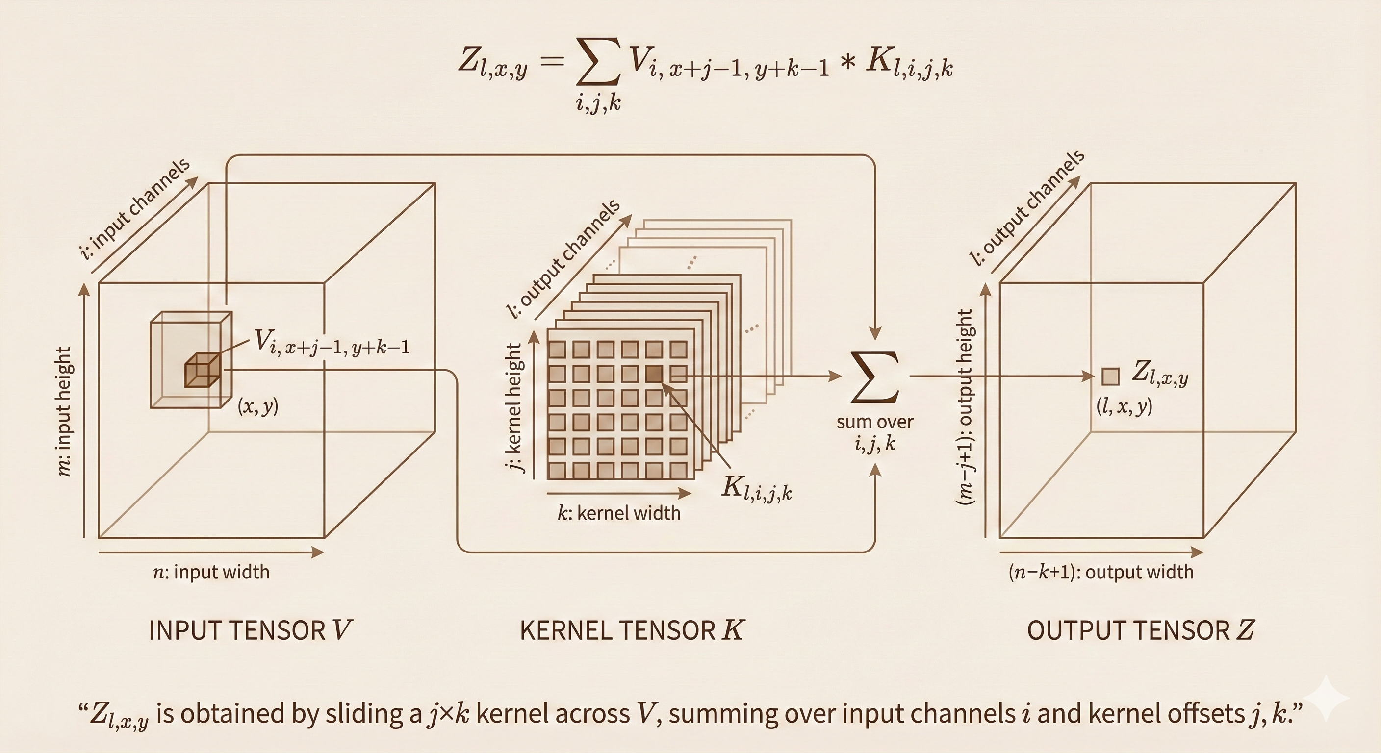 Figure: Multi-channel convolution operation - each output channel is computed by convolving all input channels with their respective kernels and summing the results.
3. Downsampling with Stride
When stride \(s \neq 1\), the convolution formula becomes:
\[ Z_{l,x,y} = \sum_{i,j,k} V_{i,(x-1)s+j,(y-1)s+k} \, K_{l,i,j,k} \tag{9.8} \]
Effect: - Stride \(s = 1\): No downsampling (default) - Stride \(s = 2\): Output dimensions halved - Stride \(s > 1\): Output dimensions reduced by factor of \(s\)
Output size with stride:
\[ \text{Output height} = \left\lfloor \frac{m - j}{s} \right\rfloor + 1 \]
\[ \text{Output width} = \left\lfloor \frac{n - k}{s} \right\rfloor + 1 \]
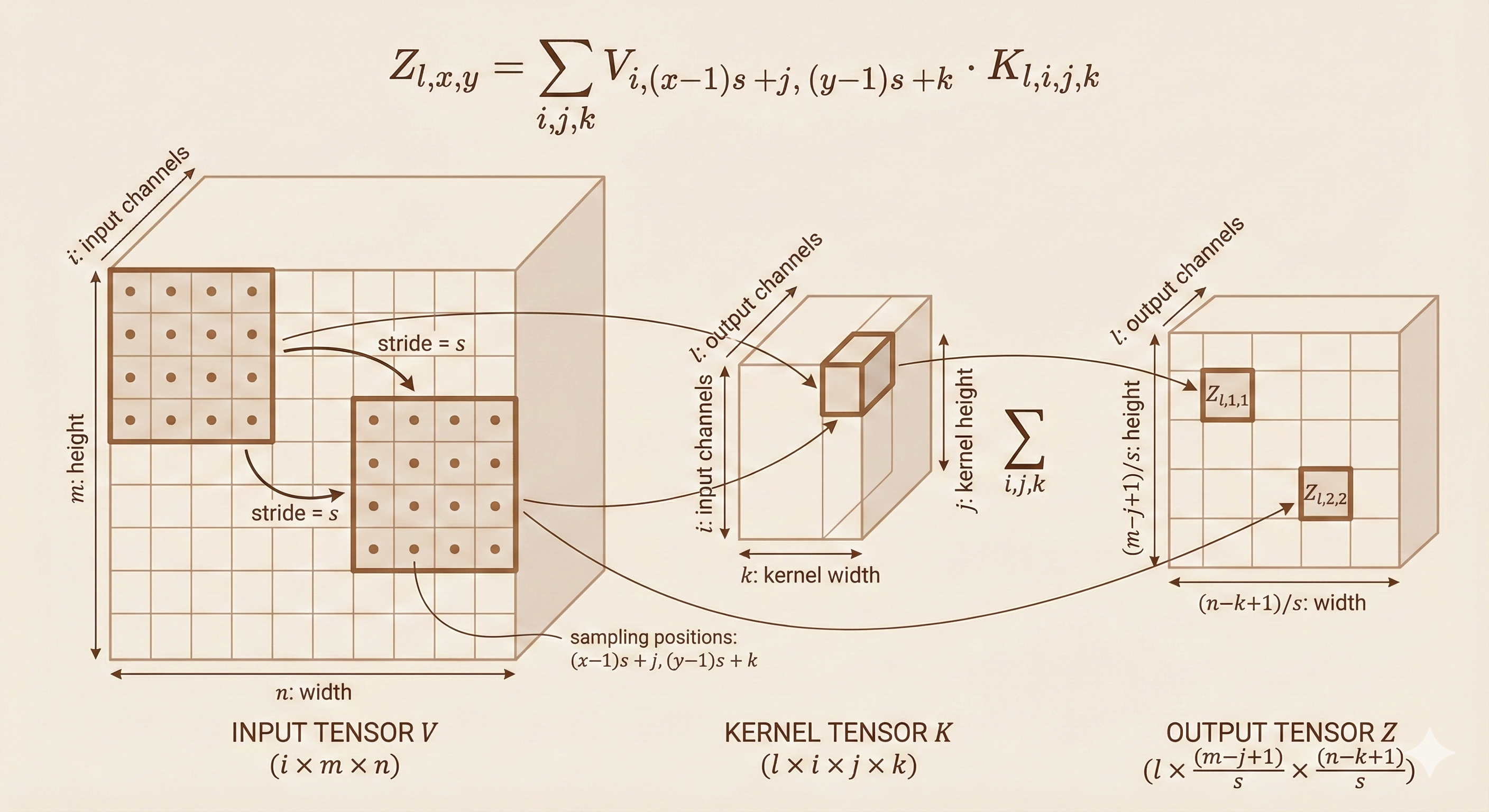 Figure: Strided convolution with stride s=2 - the kernel moves by 2 pixels at a time instead of 1, reducing the output spatial dimensions.
4. Padding Strategies
Without padding, the spatial dimensions shrink with each layer. Padding addresses this by adding borders around the input.
Valid Convolution (No Padding)
- Padding: 0
- Output height: \(h \to h - j + 1\)
- Output width: \(w \to w - k + 1\)
- Use case: When dimension reduction is acceptable
Same Convolution (Preserve Size)
- Padding: Add \(\frac{j-1}{2}\) rows to top/bottom, \(\frac{k-1}{2}\) columns to left/right
- Output height: \(h \to h\)
- Output width: \(w \to w\)
- Use case: Deep networks where preserving dimensions is important
- Note: Requires \(j\) and \(k\) to be odd
Full Convolution (Maximum Padding)
- Padding: Add \(j-1\) rows to top/bottom, \(k-1\) columns to left/right
- Output height: \(h \to h + j - 1\)
- Output width: \(w \to w + k - 1\)
- Use case: Transposed convolution (upsampling)
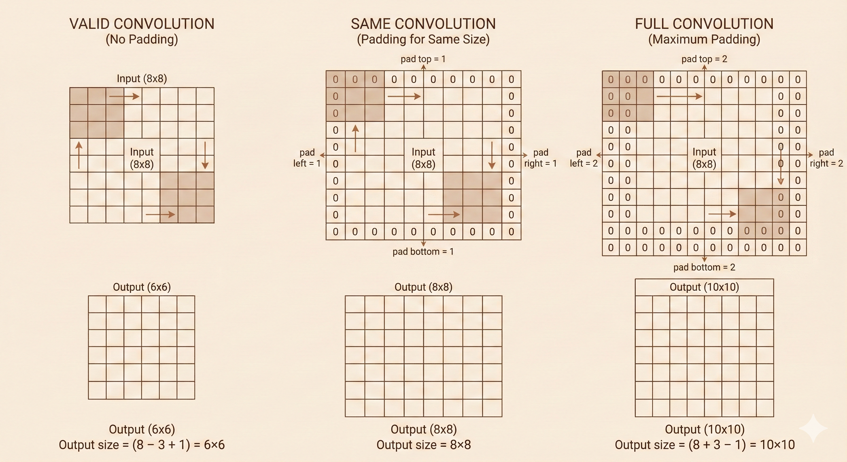 Figure: Three padding strategies - valid (no padding), same (preserve size), and full (maximum padding) convolution.
5. Local Connected Layer
Unlike standard convolution, the local connected layer does not share parameters across spatial positions.
Parameter Tensor
\[ W \in \mathbb{R}^{l \times x \times y \times i \times j \times k} \]
Dimensions: - \(l\): output channels - \(x\): output height - \(y\): output width - \(i\): input channels - \(j\): kernel height - \(k\): kernel width
Computation Formula
\[ Z_{l,x,y} = \sum_{i,j,k} V_{i,x+j-1,y+k-1} \, W_{l,x,y,i,j,k} \tag{9.9} \]
Key difference: Each spatial position \((x, y)\) has its own unique kernel weights \(W_{l,x,y,i,j,k}\) instead of sharing weights across positions.
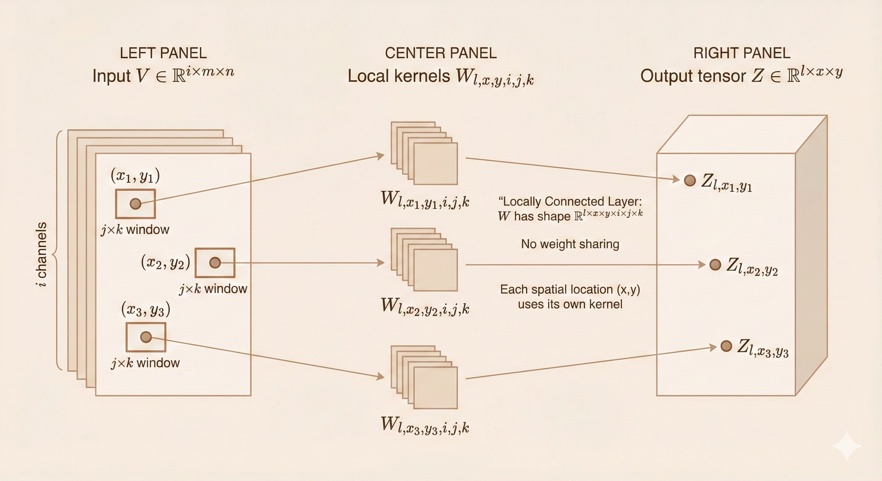 Figure: Local connected layer - each spatial position uses different weights (no parameter sharing), requiring a 6-dimensional weight tensor.
Trade-off: - Advantage: More flexible, can learn position-specific features - Disadvantage: Many more parameters, loses translation equivariance
6. Tiled Convolution
Tiled convolution is a compromise between standard convolution and locally connected layers.
Concept
Tiled convolution introduces a hyperparameter \(t\). In each spatial direction, the layer cycles through \(t\) different kernels periodically.
Parameter Tensor
\[ K \in \mathbb{R}^{l \times t \times t \times i \times j \times k} \]
Computation Formula
\[ Z_{l,x,y} = \sum_{i,j,k} V_{i,x+j-1,y+k-1} \, K_{l,(x \bmod t)+1,(y \bmod t)+1,i,j,k} \tag{9.10} \]
How it works: - At position \((x, y)\), use kernel indexed by \((x \bmod t, y \bmod t)\) - Kernels repeat in a tiled pattern across the spatial dimensions - With \(t=1\): Reduces to standard convolution (full sharing) - With \(t = \text{output size}\): Becomes locally connected (no sharing)
Modern practice: Tiled convolution is rarely used today. Modern architectures rely on more effective alternatives such as group convolution, depthwise convolution, and dilated convolution.
7. Gradient Computation for Backpropagation
To train a convolutional network \(c(K, V, s)\) with loss \(J(K, V)\), we need gradients with respect to both kernel \(K\) and input \(V\).
Gradient Tensor
Given:
\[ G_{l,x,y} = \frac{\partial}{\partial Z_{l,x,y}} J(V, K) \]
This is the gradient flowing back from the loss to the output \(Z\).
Gradient with Respect to Kernel
\[ g(G, V, s)_{l,i,j,k} = \frac{\partial}{\partial K_{l,i,j,k}} J(V, K) = \sum_{x,y} G_{l,x,y} \, V_{i,(x-1)s+j,(y-1)s+k} \tag{9.11} \]
Interpretation: The gradient for each kernel element is computed by correlating the output gradient \(G\) with the corresponding input regions.
Gradient with Respect to Input
We also need gradients with respect to input \(V\) for backpropagation through earlier layers:
\[ h(K, G, s)_{i,x,y} = \frac{\partial}{\partial V_{i,x,y}} J(V, K) \tag{9.12} \]
Full formula:
\[ H_{i,a,b} = \sum_{l} \sum_{x} \sum_{y} K_{l,i,a-(x-1)s,b-(y-1)s} \, G_{l,x,y} \tag{9.13} \]
Interpretation: The gradient for each input element is computed by convolving the flipped kernel with the output gradient.
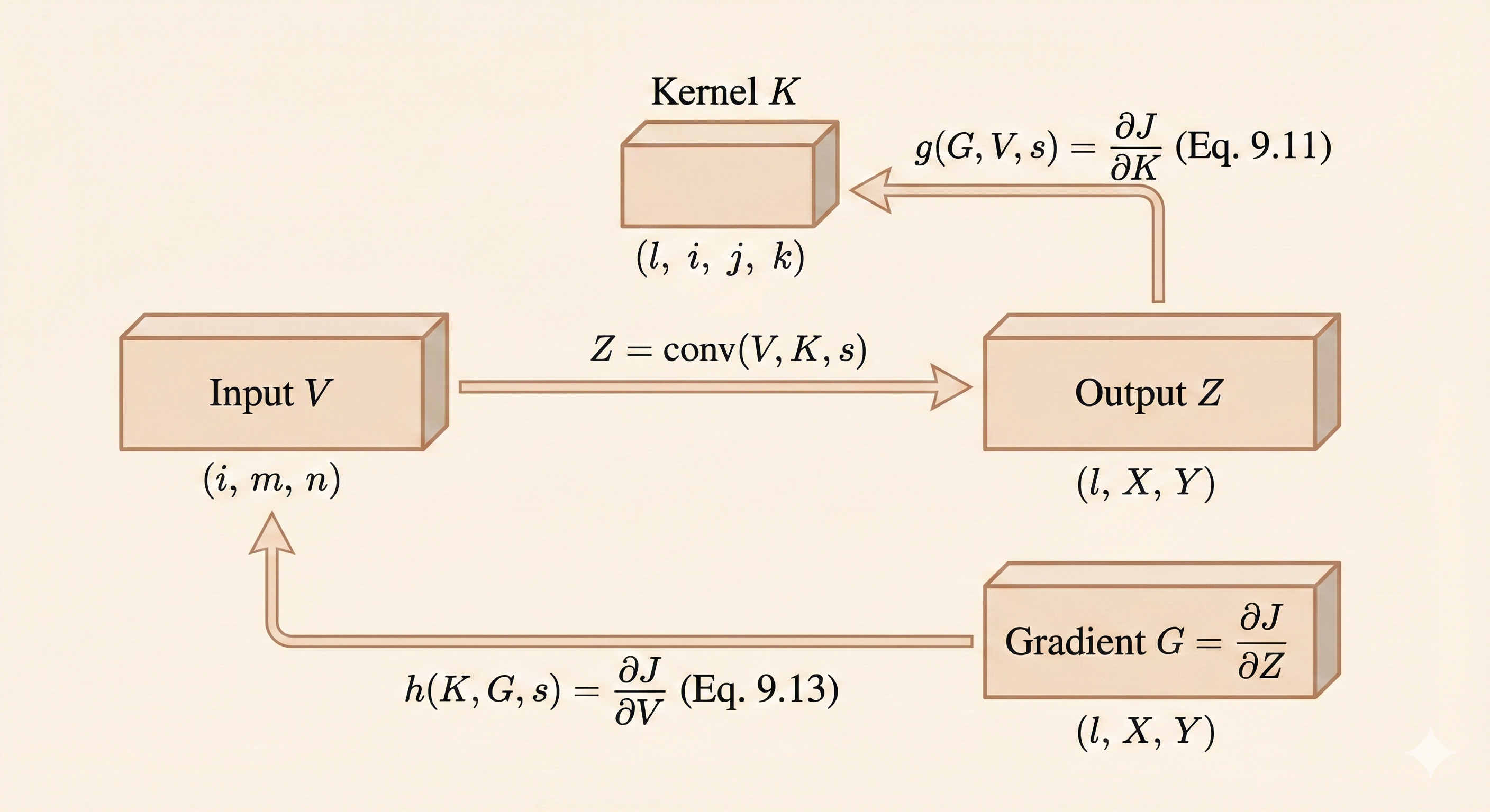 Figure: Gradient computation - gradients flow backward through the convolution operation, requiring correlation for kernel gradients and convolution with flipped kernel for input gradients.
8. Encoder-Decoder Networks
In an encoder-decoder architecture, \(h(K, H, s)\) provides the backward pass of the convolution, propagating gradients from the decoder output back to the encoder input.
\[ R = h(K, H, s) \]
Training requirements: - To train the encoder: Need gradients of \(R\) (the reconstructed input) - To train the decoder: Need gradients of \(K\) (the decoder kernel)
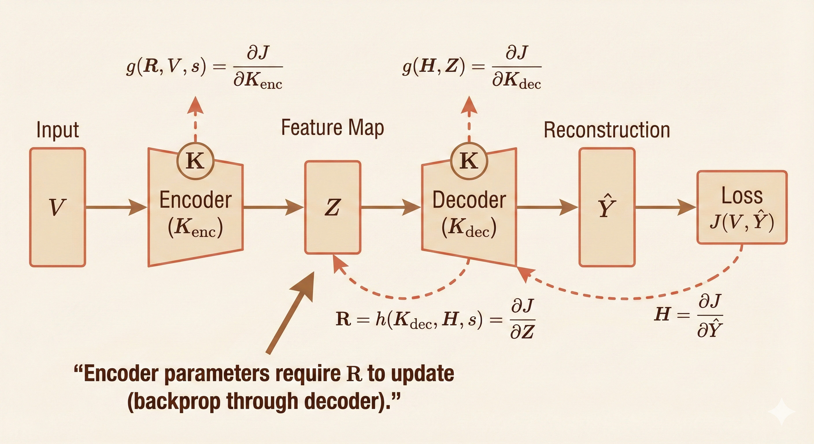 Figure: Encoder-decoder network - the encoder compresses the input through convolutions, and the decoder reconstructs it. Gradients flow backward through both parts using the formulas above.
Applications: - Image segmentation - Autoencoders - Image-to-image translation - Super-resolution
Summary
| Concept | Key Formula | Key Idea |
|---|---|---|
| Math Convolution | \((f * g)(t) = \sum_\tau f(\tau) g(t-\tau)\) | Commutative, invertible |
| DL Convolution | \((f \star g)(t) = \sum_\tau f(t+\tau) g(\tau)\) | Cross-correlation, non-commutative |
| Multi-channel | \(Z_{l,x,y} = \sum_{i,j,k} V_{i,x+j-1,y+k-1} K_{l,i,j,k}\) | Sum over input channels |
| Stride | \(Z_{l,x,y} = \sum_{i,j,k} V_{i,(x-1)s+j,(y-1)s+k} K_{l,i,j,k}\) | Downsampling |
| Padding | Valid/Same/Full | Control output size |
| Local Connected | \(W \in \mathbb{R}^{l \times x \times y \times i \times j \times k}\) | No parameter sharing |
| Tiled Conv | Kernel indexed by \((x \bmod t, y \bmod t)\) | Periodic parameter sharing |
| Kernel Gradient | \(\nabla_K J = \sum_{x,y} G_{l,x,y} V_{i,(x-1)s+j,(y-1)s+k}\) | Correlation of output gradient with input |
| Input Gradient | \(\nabla_V J = \sum_{l,x,y} K_{l,i,a-(x-1)s,b-(y-1)s} G_{l,x,y}\) | Convolution with flipped kernel |
Key takeaways: - Deep learning uses cross-correlation (not true mathematical convolution) - Stride enables downsampling without pooling - Padding controls output spatial dimensions - Gradient computation requires different operations for kernel vs input - Modern architectures favor standard convolution over tiled or locally connected variants