---
title: "Goodfellow Deep Learning — Deep Learning Book 6.4: Architecture Design - Depth vs Width"
author: "Chao Ma"
date: "2025-09-30"
categories: ["Deep Learning", "Neural Networks", "Architecture Design"]
code-fold: true
code-summary: "Show code"
---
*This recap of Deep Learning Chapter 6.4 explores how network architecture—depth versus width—fundamentally shapes what neural networks can learn and how efficiently they learn it.*
📓 **For a deeper dive with additional exercises and analysis**, see the [complete notebook on GitHub](https://github.com/ickma2311/foundations/blob/main/deep_learning/chapter6/6.4/exercises.ipynb).
## The Architecture Question: Deep or Wide?
When designing a neural network, one of the most fundamental decisions is choosing between depth (many layers) and width (many units per layer). Should you build a shallow network with many units, or a deep network with fewer units per layer?
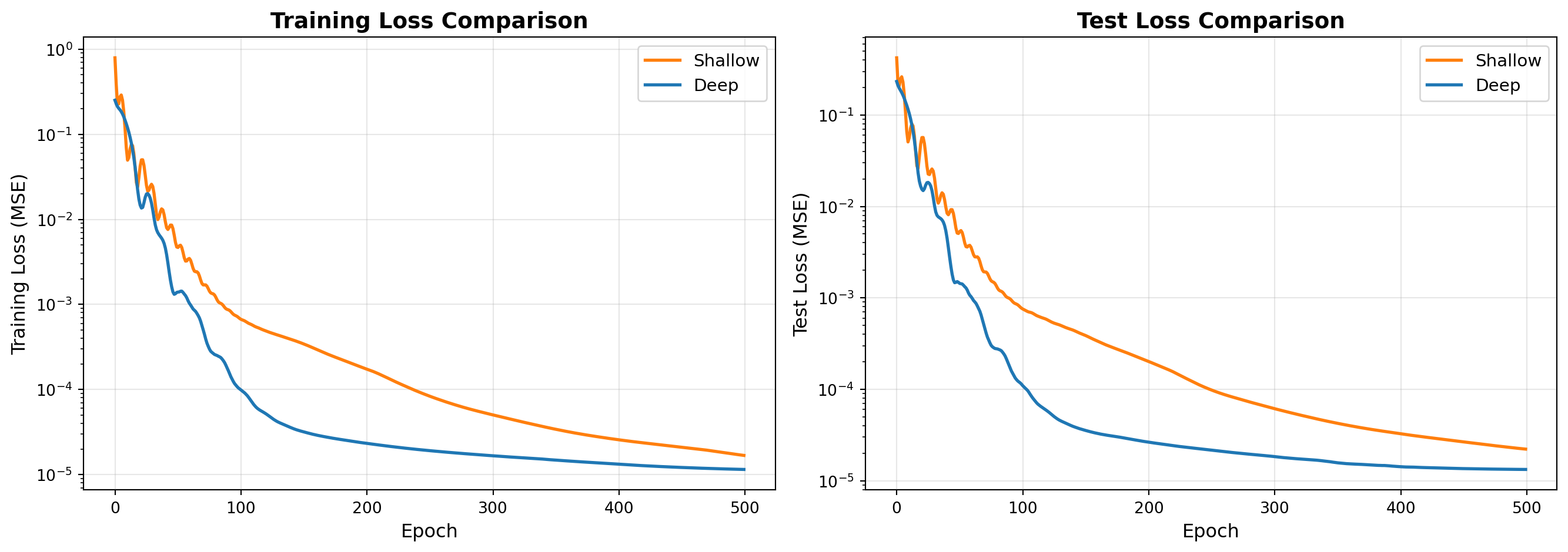
The answer reveals something profound about how neural networks represent functions: **deep networks can achieve exponentially greater expressiveness than shallow networks with the same number of parameters**. This isn't just theoretical—it has practical implications for model efficiency and performance.
### Quick Reference: Understanding Depth vs Width
For context on the fundamental concepts of network architecture, see the [Architecture Design summary](https://github.com/ickma2311/foundations/blob/main/deep_learning/chapter6/6.4/architecture_design.md).
**Key insight**: A deep ReLU network with $n$ units per layer and depth $L$ can create $\mathcal{O}(n^L)$ distinct linear regions in the input space. A shallow network would need exponentially many units ($\mathcal{O}(n^L)$ units in a single layer) to achieve the same expressiveness.
| **Architecture** | **Characteristic** | **Advantage** | **Challenge** |
|------------------|-------------------|---------------|---------------|
| **Deep** (many layers) | Hierarchical feature reuse | Exponential expressiveness with fewer parameters | Harder to optimize (vanishing/exploding gradients) |
| **Wide** (many units per layer) | Increased capacity per layer | Easier optimization | Parameter inefficient; requires exponentially more units |
## 🔬 Experiment: Shallow vs Deep Network Comparison
Let's explore whether depth provides an advantage in practice by comparing two networks:
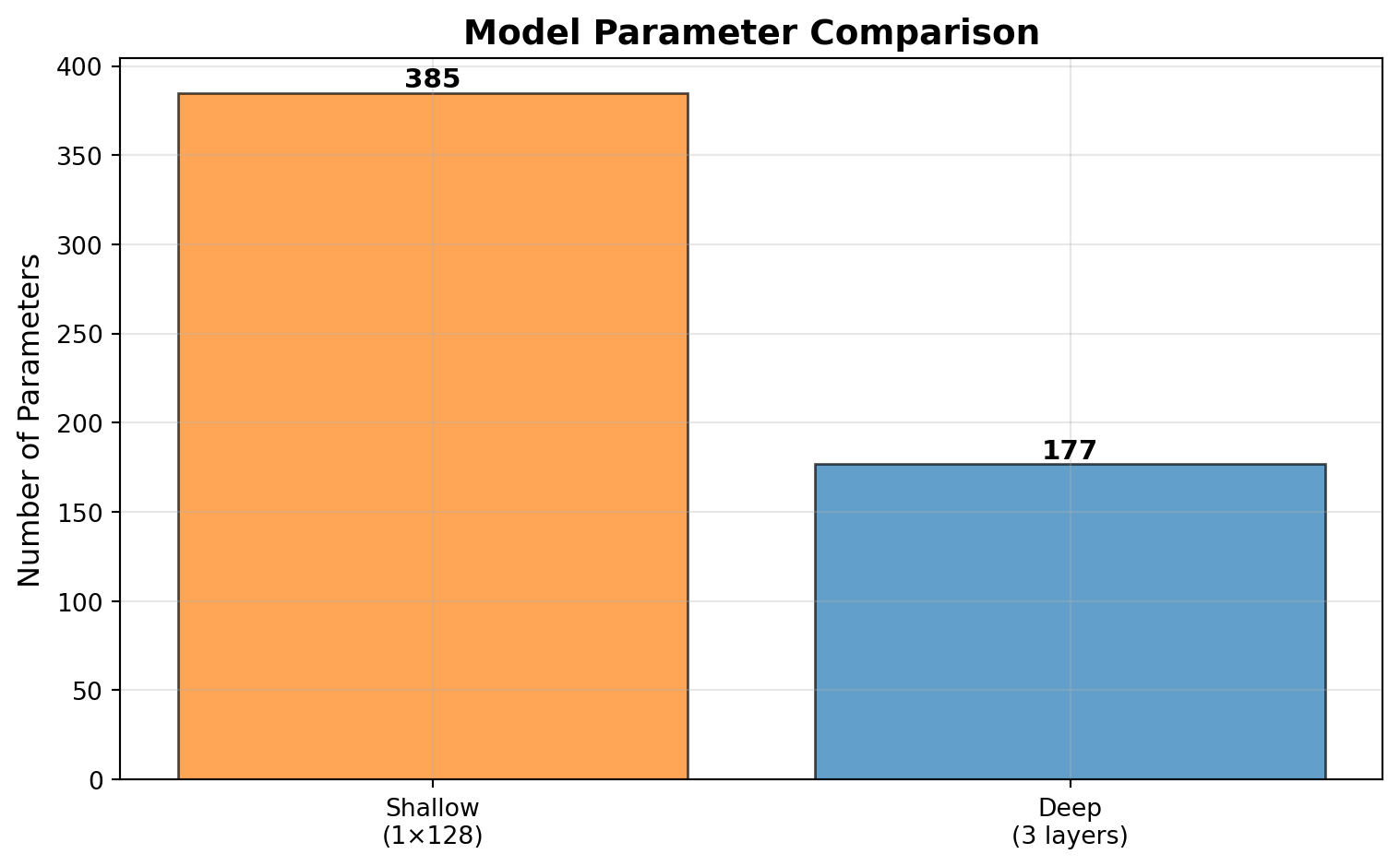
- **Shallow Network**: 1 hidden layer with 128 units
- **Deep Network**: 3 hidden layers (16 → 8 → output)
Both networks are trained on the same regression task: $y = \sin^2(x) + x^3$
```{python}
import numpy as np
import matplotlib.pyplot as plt
import torch
import torch.nn as nn

# Set random seed for reproducibility
np.random.seed(42)
torch.manual_seed(42)

# Configure plotting
plt.rcParams['figure.facecolor'] = 'white'
plt.rcParams['axes.facecolor'] = 'white'
plt.rcParams['axes.grid'] = True
plt.rcParams['grid.alpha'] = 0.3

print("✓ Setup complete")
```
### Step 1: Generate Training and Test Data
```{python}
# Training data
x_train = np.random.rand(200, 1)
y_train = np.square(np.sin(x_train)) + np.power(x_train, 3)

# Test data
x_test = np.random.rand(100, 1)
y_test = np.square(np.sin(x_test)) + np.power(x_test, 3)

# Convert to PyTorch tensors
x_train_tensor = torch.FloatTensor(x_train)
y_train_tensor = torch.FloatTensor(y_train)
x_test_tensor = torch.FloatTensor(x_test)
y_test_tensor = torch.FloatTensor(y_test)

print(f"Training samples: {len(x_train)}")
print(f"Test samples: {len(x_test)}")
print(f"Input range: [{x_train.min():.2f}, {x_train.max():.2f}]")
print(f"Target range: [{y_train.min():.2f}, {y_train.max():.2f}]")
```
### Step 2: Define Model Architectures
```{python}
# Shallow model: 1 hidden layer with 128 units
shallow_model = nn.Sequential(
    nn.Linear(1, 128),
    nn.ReLU(),
    nn.Linear(128, 1)
)

# Deep model: 3 hidden layers (16 → 8 → output)
deep_model = nn.Sequential(
    nn.Linear(1, 16),
    nn.ReLU(),
    nn.Linear(16, 8),
    nn.ReLU(),
    nn.Linear(8, 1)
)

print("✓ Models created")
print(f"\nShallow model architecture:")
print(shallow_model)
print(f"\nDeep model architecture:")
print(deep_model)
```
### Step 3: Count Parameters
How many trainable parameters does each architecture use?
```{python}
def count_parameters(model):
    """Count total trainable parameters in a model"""
    return sum(p.numel() for p in model.parameters() if p.requires_grad)

shallow_params = count_parameters(shallow_model)
deep_params = count_parameters(deep_model)

print("Parameter Counts:")
print("-" * 50)
print(f"Shallow model (1 layer × 128 units): {shallow_params:,} parameters")
print(f"Deep model (3 layers):                {deep_params:,} parameters")
print("-" * 50)
print(f"Ratio (shallow/deep): {shallow_params/deep_params:.2f}x")

# Visualize parameter counts
fig, ax = plt.subplots(figsize=(8, 5))
models = ['Shallow\n(1×128)', 'Deep\n(3 layers)']
params = [shallow_params, deep_params]
colors = ['#ff7f0e', '#1f77b4']

bars = ax.bar(models, params, color=colors, alpha=0.7, edgecolor='black')
ax.set_ylabel('Number of Parameters', fontsize=12)
ax.set_title('Model Parameter Comparison', fontsize=14, fontweight='bold')
ax.grid(axis='y', alpha=0.3)

# Add value labels on bars
for bar, param in zip(bars, params):
    height = bar.get_height()
    ax.text(bar.get_x() + bar.get_width()/2., height,
            f'{param:,}',
            ha='center', va='bottom', fontsize=11, fontweight='bold')

plt.tight_layout()
plt.show()
```
### Step 4: Train Both Models
```{python}
# Training configuration
n_epochs = 500
learning_rate = 0.01
loss_fn = nn.MSELoss()

# Track training history
history = {
    'Shallow': {'train_loss': [], 'test_loss': []},
    'Deep': {'train_loss': [], 'test_loss': []}
}

models = {
    'Shallow': shallow_model,
    'Deep': deep_model
}

# Train each model
for name, model in models.items():
    optimizer = torch.optim.Adam(model.parameters(), lr=learning_rate)

    for epoch in range(n_epochs):
        # Training
        model.train()
        y_pred = model(x_train_tensor)
        loss = loss_fn(y_pred, y_train_tensor)

        optimizer.zero_grad()
        loss.backward()
        optimizer.step()

        history[name]['train_loss'].append(loss.item())

        # Evaluation on test set
        model.eval()
        with torch.no_grad():
            y_test_pred = model(x_test_tensor)
            test_loss = loss_fn(y_test_pred, y_test_tensor).item()
            history[name]['test_loss'].append(test_loss)

    print(f"✓ {name} model trained")

print("\n✓ Training complete")
```
### Step 5: Compare Model Performance
```{python}
fig, axes = plt.subplots(1, 2, figsize=(14, 5))
colors = {'Shallow': '#ff7f0e', 'Deep': '#1f77b4'}

# Plot training loss
for name, data in history.items():
    axes[0].plot(data['train_loss'], label=name, linewidth=2, color=colors[name])

axes[0].set_xlabel('Epoch', fontsize=12)
axes[0].set_ylabel('Training Loss (MSE)', fontsize=12)
axes[0].set_title('Training Loss Comparison', fontsize=14, fontweight='bold')
axes[0].legend(fontsize=11)
axes[0].grid(True, alpha=0.3)
axes[0].set_yscale('log')

# Plot test loss
for name, data in history.items():
    axes[1].plot(data['test_loss'], label=name, linewidth=2, color=colors[name])

axes[1].set_xlabel('Epoch', fontsize=12)
axes[1].set_ylabel('Test Loss (MSE)', fontsize=12)
axes[1].set_title('Test Loss Comparison', fontsize=14, fontweight='bold')
axes[1].legend(fontsize=11)
axes[1].grid(True, alpha=0.3)
axes[1].set_yscale('log')

plt.tight_layout()
plt.show()

# Print final metrics
print("\nFinal Performance (after {} epochs):".format(n_epochs))
print("-" * 70)
print(f"{'Model':<15} {'Parameters':<15} {'Train Loss':<15} {'Test Loss':<15}")
print("-" * 70)
for name in models.keys():
    params = count_parameters(models[name])
    train_loss = history[name]['train_loss'][-1]
    test_loss = history[name]['test_loss'][-1]
    print(f"{name:<15} {params:<15,} {train_loss:<15.6f} {test_loss:<15.6f}")
```
---
*This experiment demonstrates the practical implications of depth versus width in neural network architecture design, showing how deeper networks can achieve competitive performance with fewer parameters.*

