Goodfellow Deep Learning — Chapter 10.2: Recurrent Neural Networks
RNN Architecture
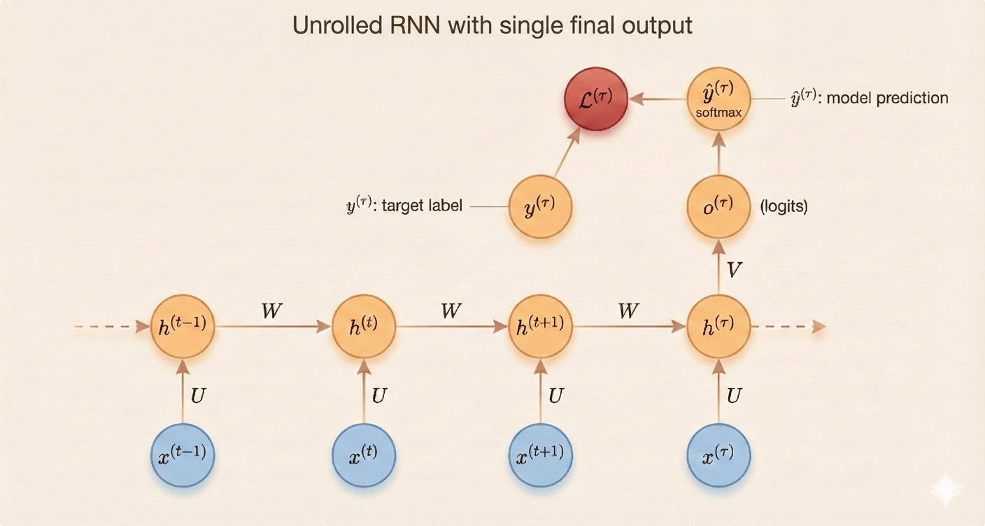
Assume the output is discrete (e.g., predicting the next token), and the activation function is tanh.
\[ a^{(t)} = Wh^{(t-1)} + Ux^{(t)} + b \tag{10.8} \]
\[ h^{(t)} = \tanh(a^{(t)}) \tag{10.9} \]
\[ o^{(t)} = Vh^{(t)} + c \tag{10.10} \]
\[ \hat{y}^{(t)} = \text{softmax}(o^{(t)}) \tag{10.11} \]
Parameters:
- \(W\): weight matrix connecting hidden state \(h^{(t-1)}\) to next hidden state
- \(U\): weight matrix connecting input \(x\) to hidden state
- \(b\): bias for hidden state
- \(\tanh\): activation function
- \(V\): weight matrix connecting hidden layer \(h^{(t)}\) to output
- \(c\): output bias
The loss of a given input sequence x is the sum of the prediction losses at all time steps:
\[ L(\{x^{(1)},...,x^{(\tau)}\}, \{y^{(1)},...,y^{(\tau)}\}) = \sum_t L^{(t)} = -\sum_t \log p_{\text{model}}(y^{(t)} | \{x^{(1)},...,x^{(\tau)}\}) \tag{10.12-10.14} \]
Complexity:
- Time complexity is \(O(\tau)\): Both forward propagation and back-propagation through time (BPTT) must proceed sequentially across all time steps and cannot be parallelized.
- Space complexity is \(O(\tau)\): BPTT requires storing all intermediate hidden states and activations for all time steps.
Teacher Forcing and Networks with Output Recurrence
In an output-recurrent network, there is no hidden-to-hidden connection. The hidden state at time \(t\) depends only on the current input and the output from the previous time step:
\[ h^{(t)} = f(Ux^{(t)} + Wy^{(t-1)}) \]
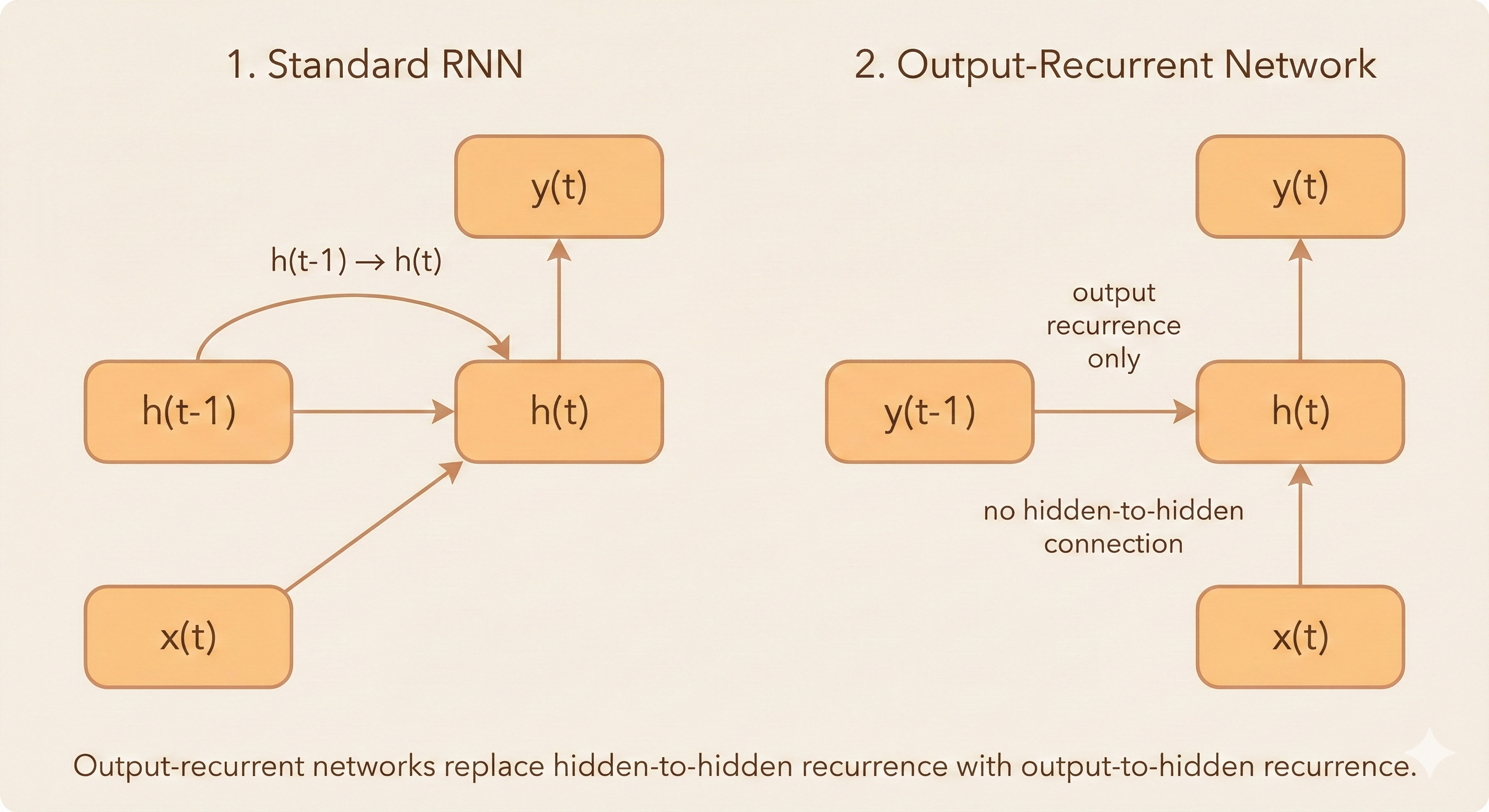
Teacher Forcing:
During training, the model does not use its own approximate predictions as inputs. Instead, it receives the ground truth from the previous time step, a technique known as teacher forcing.
This allows training to be parallelized because each time step no longer needs to wait for the output of the previous step.
The conditional log-likelihood is:
\[ \log p(y^{(1)}, y^{(2)} | x^{(1)}, x^{(2)}) = \log p(y^{(2)} | y^{(1)}, x^{(1)}, x^{(2)}) + \log p(y^{(1)} | x^{(1)}, x^{(2)}) \tag{10.16} \]
Training vs. Inference:
- During training: the model uses the ground-truth output \(y^{(t)}\) as the input for the next time step
- At test time: the ground truth is not available, so the model feeds its own prediction \(\hat{y}^{(t)}\) into the next step instead
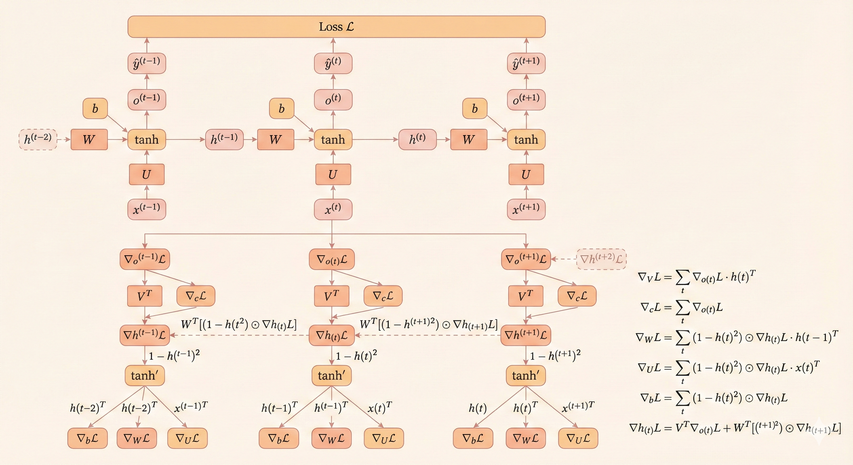
Gradient of RNN (Back-Propagation Through Time)
The partial derivative of \(L^{(t)}\) with respect to \(L\) is 1:
\[ L = L^{(1)} + ... + L^{(\tau)}, \quad \frac{\partial L}{\partial L^{(t)}} = 1 \tag{10.17} \]
Suppose the output \(o^{(t)}\) is the parameter of softmax. For each \(i, t\) (where \(i\) is the index of y labels and \(t\) is the time step):
\[ (\nabla_{o^{(t)}} L)_i = \frac{\partial L}{\partial o_i^{(t)}} = \frac{\partial L}{\partial L^{(t)}} \frac{\partial L^{(t)}}{\partial o_i^{(t)}} = \hat{y}_i^{(t)} - \mathbf{1}_{i=y^{(t)}} \tag{10.18} \]
The gradient of softmax is: \(\boxed{\frac{\partial L}{\partial o_i} = \hat{y}_i - \mathbf{1}_{i=y}}\)
Gradient at Last Time Step
At the last step \(\tau\), the hidden unit \(h\) has no future step, so the gradient is:
\[ \nabla_{h^{(\tau)}} L = V^\top \nabla_{o^{(\tau)}} L \tag{10.19} \]
since \(o^{(\tau)} = Vh^{(\tau)} + c\).
Back-Propagation from \(\tau-1\) to 1
For all steps from \(\tau-1 \to 1\), \(h^{(t)}\) has 2 downstream nodes: \(o^{(t)}\) and \(h^{(t+1)}\).
The gradient is:
\[ \nabla_{h^{(t)}} L = \left(\frac{\partial h^{(t+1)}}{\partial h^{(t)}}\right)^\top (\nabla_{h^{(t+1)}} L) + \left(\frac{\partial o^{(t)}}{\partial h^{(t)}}\right)^\top \nabla_{o^{(t)}} L \tag{10.20} \]
Where:
- \(\frac{\partial h^{(t+1)}}{\partial h^{(t)}}\): Jacobian mapping changes in \(h^{(t)}\) to changes in \(h^{(t+1)}\)
- From: \(h^{(t+1)} = \tanh(Wh^{(t)} + Ux^{(t+1)} + b)\)
- \(\frac{\partial o^{(t)}}{\partial h^{(t)}}\): Jacobian mapping changes in \(h^{(t)}\) to changes in \(o^{(t)}\)
- From: \(o^{(t)} = Vh^{(t)} + c\)
\[ \nabla_{h^{(t)}} L = W^\top \operatorname{diag}(1-(h^{(t+1)})^2) \nabla_{h^{(t+1)}} L + V^\top \nabla_{o^{(t)}} L \tag{10.21} \]
Gradients of Parameters
Bias \(c\) (forward gradient is 1):
\[ \nabla_c L = \sum_t \left(\frac{\partial o^{(t)}}{\partial c}\right)^\top \nabla_{o^{(t)}} L = \sum_t \nabla_{o^{(t)}} L \tag{10.22} \]
Bias \(b\) (forward gradient is \(\text{diag}(1 - (h^{(t)})^2)\)):
\[ \nabla_b L = \sum_t \left(\frac{\partial h^{(t)}}{\partial b}\right)^\top \nabla_{h^{(t)}} L = \sum_t \text{diag}(1 - (h^{(t)})^2) \nabla_{h^{(t)}} L \tag{10.23} \]
Weight \(V\) (forward gradient is \((h^{(t)})^\top\)):
\[ \nabla_V L = \sum_t \nabla_{o^{(t)}} L (h^{(t)})^\top \tag{10.24} \]
Weight \(W\) (forward gradient is \(\text{diag}(1 - (h^{(t)})^2)(h^{(t-1)})^\top\)):
\[ \nabla_W L = \sum_t \text{diag}(1 - (h^{(t)})^2) \nabla_{h^{(t)}} L (h^{(t-1)})^\top \tag{10.25} \]
Weight \(U\) (forward gradient is \(\text{diag}(1 - (h^{(t)})^2)(x^{(t)})^\top\)):
\[ \nabla_U L = \sum_t \text{diag}(1 - (h^{(t)})^2) \nabla_{h^{(t)}} L (x^{(t)})^\top \tag{10.26} \]
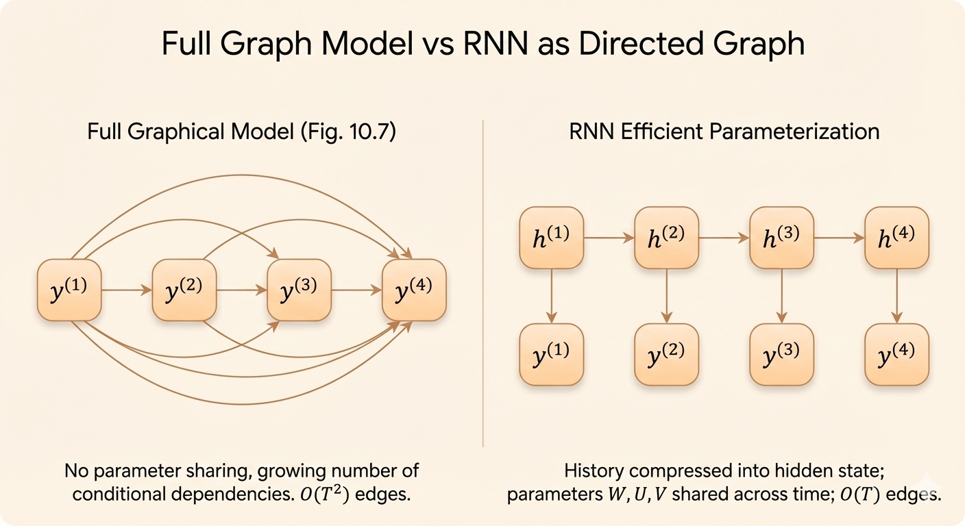
RNN as Directed Graph
The objective of RNN is to maximize the log-likelihood:
\[ \log p(y^{(t)} | x^{(1)}, ..., x^{(t)}) \tag{10.29} \]
Or the input can include the connection between the current step and the output from the previous step:
\[ \log p(y^{(t)} | x^{(1)}, ..., x^{(t)}, y^{(1)}, ..., y^{(t-1)}) \tag{10.30} \]
By only looking at sequence \(\mathbf{Y}\), the probability can be represented using chain rule:
\[ P(\mathbf{Y}) = \prod_{t=1}^{\tau} P(y^{(t)} | y^{(t-1)}, ..., y^{(1)}) \tag{10.31} \]
The negative log-likelihood is:
\[ L = \sum_t L^{(t)} \tag{10.32} \]
\[ L^{(t)} = -\log P(y^{(t)} | y^{(t-1)}, ..., y^{(1)}) \tag{10.33} \]
Parameter Complexity:
A naive fully-connected model would need \(O(k^\tau)\) parameters. An RNN uses a fixed-size hidden state, so the number of parameters is independent of \(\tau\).
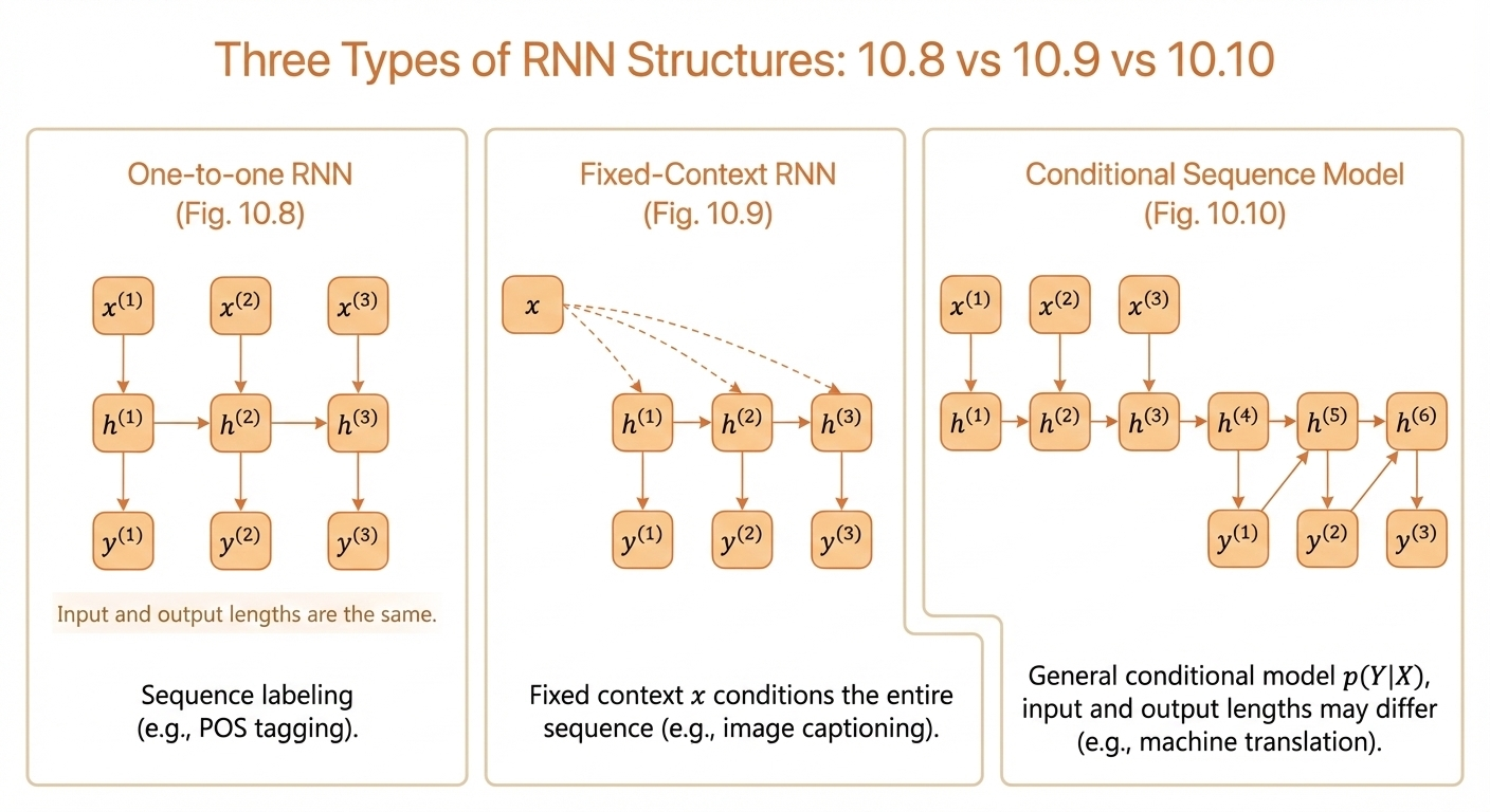
Context-Based RNN Model
Sometimes we need a fixed context \(x\) as the input (e.g., an image embedding), and we want the RNN to generate a sequence that describes the image.
More generally, the context itself can be an input sequence \(\mathbf{X} = (x^{(1)}, ..., x^{(\tau_x)})\), and the RNN models a conditional distribution over an output sequence \(\mathbf{Y} = (y^{(1)}, ..., y^{(\tau_y)})\) of possibly different length.
Example: In machine translation, the source sentence serves as the context for generating the target sentence.
Key Insights
RNNs enable sequence modeling through parameter sharing. The same weights \((W, U, V)\) are reused across all time steps, making RNNs efficient for variable-length sequences. However, this comes at the cost of sequential computation—forward and backward passes cannot be parallelized across time.
Teacher forcing accelerates training by using ground-truth outputs instead of model predictions, enabling parallel computation during training. The tradeoff is exposure bias: during inference, the model must use its own predictions, which may differ from the training distribution.
BPTT computes gradients by unfolding the network through time. The gradient at each hidden state combines contributions from both the immediate output and all future time steps, enabling the network to learn long-range dependencies (though vanishing/exploding gradients remain a challenge).