EE 364A (Convex Optimization): Lecture 1 - Introduction
Lecture Video
Mathematical Definition
Constraint Optimization Problems
Minimize \(f_0(x)\), subject to \(f_i(x) \leq b_i\), \(i=1,2,...,m\)
- \(x=(x_1,...,x_n)\): optimization variable
- \(f_0: \mathbb{R}^n \rightarrow \mathbb{R}\): objective function
- \(f_i: \mathbb{R}^n \rightarrow \mathbb{R}\), \(i=1,2,...,m\): constraint functions
Solution or optimal point \(x^*\) has the smallest value of \(f_0\) among all vectors that satisfy the constraints.
Examples
Profit Optimization
- Variables: amount invested in different assets
- Constraints: budget, max/min per asset, minimum return
- Objective: overall risk or return variance
Device Sizing in Electronic Circuits
- Variables: device width and lengths
- Constraints: manufacturing limits, timing requirements, maximum area
- Objective: power consumption
Data Fitting
- Variables: model parameters
- Constraints: prior information, parameter limits
- Objective: measure of misfit or prediction error, plus regularization term
Solving Optimization Problems
General Optimization Problems
- Difficult to solve
- Some compromise: very long computation time, or not always finding the solution
Exceptions
- Least square problems
- Linear programming
- Convex optimization
Least Squares
Minimize \(\|Ax-b\|_2^2\)
- Analytical solution: \(x^* = (A^\top A)^{-1}A^\top b\)
- Computation time: proportional to \(n^2k\) (where \(A \in \mathbb{R}^{k \times n}\))
Linear Programming
Minimize \(c^\top x\)
Subject to \(a_i^\top x \leq b_i\), \(i=1,2,...,m\)
- No analytical solution
- Reliable and efficient algorithms, software available
- Computation time: proportional to \(n^2m\) (if \(m \geq n\))
Convex Optimization
Minimize \(f_0(x)\)
Subject to \(f_i(x) \leq b_i\)
Convexity requirement: objective and constraint functions are convex:
\[f(\alpha x + \beta y) \leq \alpha f(x) + \beta f(y)\]
where \(\alpha > 0\), \(\beta > 0\), \(\alpha + \beta = 1\)
- Least squares and linear programming are special cases
- No analytical solution
- Computation time: proportional to \(\max(n^3, n^2m, F)\), where \(F\) is the cost of evaluating \(f_i\)’s and their first and second derivatives
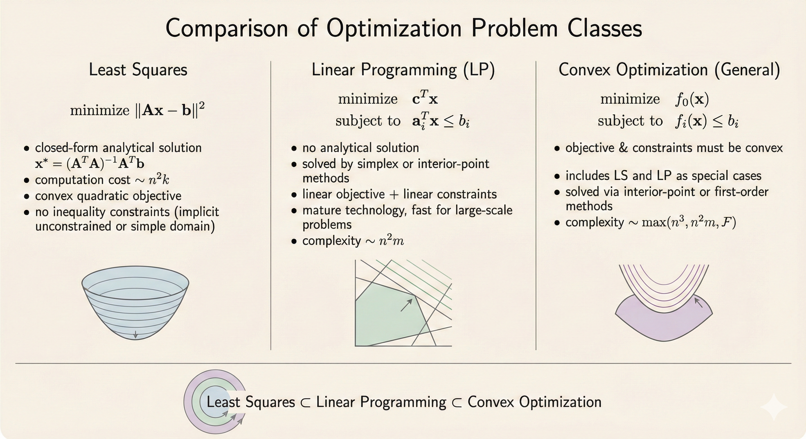 Figure: Comparing least squares, linear programming, and convex optimization in terms of complexity and solution methods. Least squares has analytical solutions, linear programming has polynomial-time algorithms, and convex optimization generalizes both while maintaining tractability.
Example: Lamp Illumination Optimization
Problem: There are \(m\) lamps illuminating \(n\) patches. The goal is to choose lamp powers so that all patches have illumination \(I_k\) close to a desired value \(I_{\text{des}}\), by minimizing the maximum log-illumination error, subject to power constraints.
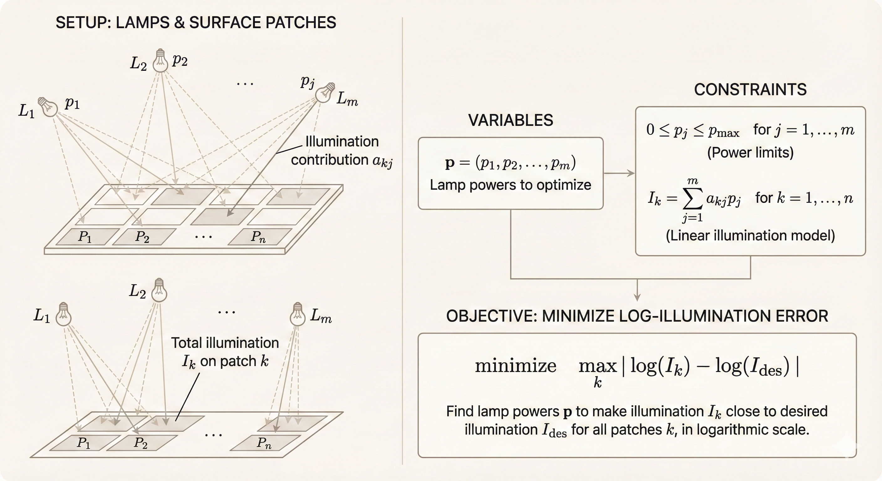 Figure: Lamp illumination optimization problem. Given m lamps and n patches, find lamp powers that achieve uniform illumination across all patches while respecting power constraints. This is a convex optimization problem that can be solved efficiently.
Key Insight
Convex optimization bridges the gap between tractable special cases and general nonlinear programming. Least squares problems have closed-form solutions but are limited in expressiveness. General optimization is flexible but computationally intractable. Convex optimization occupies a sweet spot: it generalizes least squares and linear programming while maintaining polynomial-time solvability through interior-point methods. This makes convex optimization the foundation for practical applications in machine learning, control systems, signal processing, and engineering design.