Lecture 9: Four Ways to Solve Least Squares Problems
Overview
This lecture presents four methods for solving least squares problems \(Ax = b\) when \(A\) has no inverse, exploring the connections between pseudo-inverse, normal equations, and projection geometry.
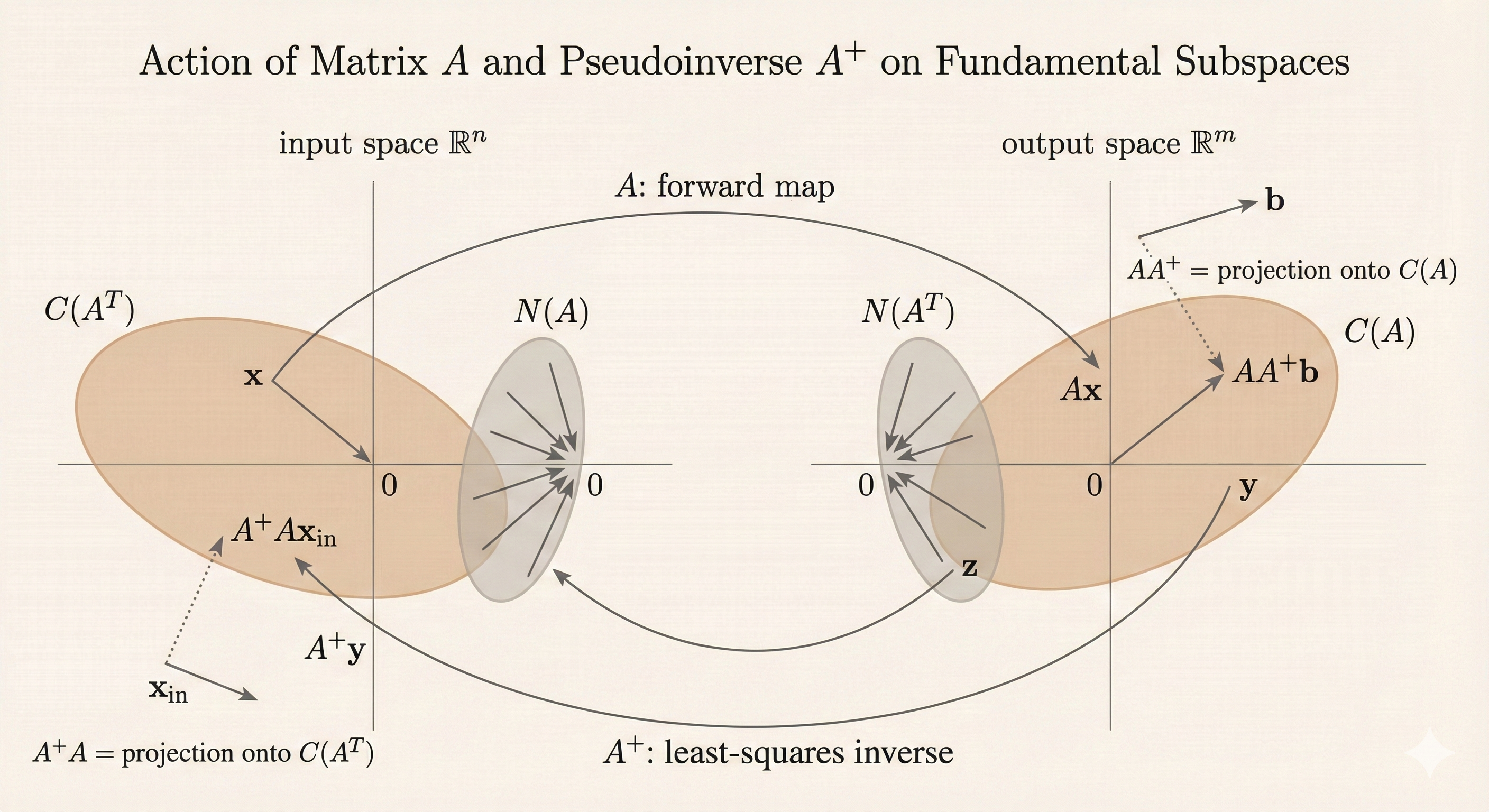
Projection Matrices
Understanding projections is key to least squares:
- \(A^+A\): Projection onto row space \(C(A^T)\)
- If \(x\) is in the row space, we get \(x\) back
- If \(x\) is in the null space, it gets mapped to \(0\)
- \(AA^+\): Projection onto column space \(C(A)\)
- Projects vectors onto the column space of \(A\)
 Figure: The four fundamental subspaces and how projection matrices \(A^+A\) and \(AA^+\) map between them.
Method 1: Pseudo-Inverse
Using the SVD decomposition \(A = U\Sigma V^T\):
For invertible matrices: \[A^{-1} = V\Sigma^{-1}U^T\]
For non-invertible matrices: \[A^+ = V\Sigma^+ U^T\]
where \(\Sigma^+\) inverts only the non-zero singular values:
\[ \Sigma^+ = \begin{bmatrix} \frac{1}{\sigma_1} & 0 & \cdots & 0 \\ 0 & \frac{1}{\sigma_2} & \cdots & 0 \\ \vdots & \vdots & \ddots & \vdots \end{bmatrix} \]
Solution: \(\hat{x} = A^+ b\)
Method 2: Normal Equations
Solve \(A^T A \hat{x} = A^T b\) when \(A\) is \(m \times n\) with rank \(r\).
Linear Regression Example
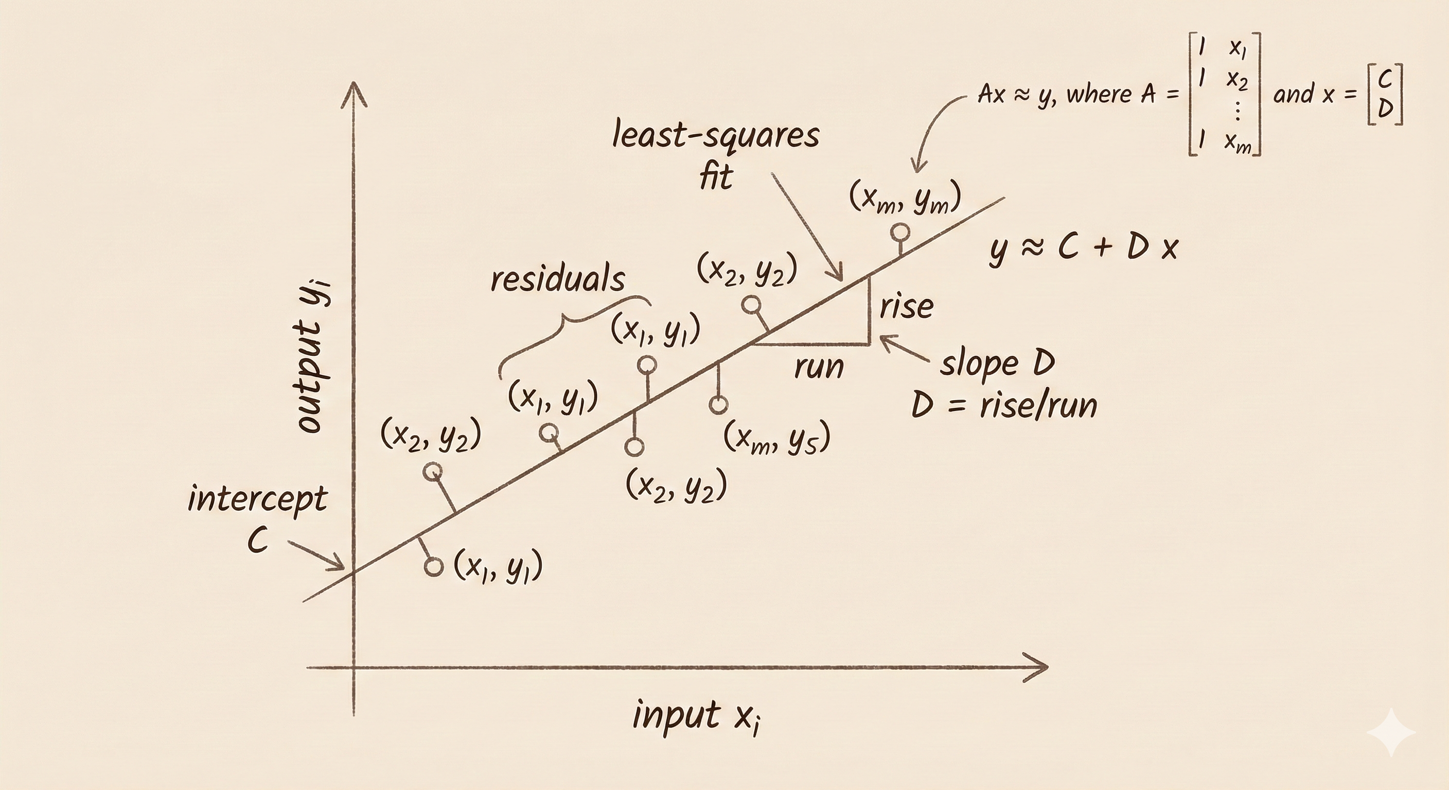
Given data points \((x_1, y_1), (x_2, y_2), \ldots, (x_m, y_m)\), we want to find \(C, D\) such that:
\[C + Dx \approx y\]
Build the matrix: \[A = \begin{bmatrix} 1 & x_1 \\ 1 & x_2 \\ \vdots & \vdots \\ 1 & x_m \end{bmatrix}, \quad A\begin{bmatrix}C \\ D\end{bmatrix} = C\begin{bmatrix}1 \\ 1 \\ \vdots \\ 1\end{bmatrix} + D\begin{bmatrix}x_1 \\ x_2 \\ \vdots \\ x_m\end{bmatrix} \]
 Figure: Setting up the least squares problem for linear regression—finding the line that best fits the data points.
Three Approaches to the Solution
1. Algebraic Approach
Minimize \(\|Ax - b\|_2^2\):
\[ \|Ax - b\|_2^2 = (Ax - b)^T(Ax - b) = x^T A^T A x - 2x^T A^T b + b^T b \]
Gradient: \[\nabla_x \|Ax - b\|_2^2 = 2A^T A x - 2A^T b\]
Setting gradient to zero: \[A^T A \hat{x} = A^T b\]
2. Geometric Approach
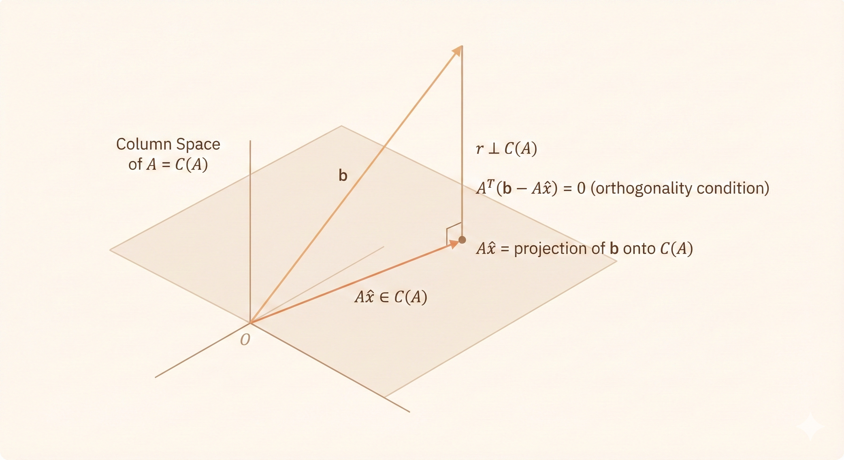
- The vector \(Ax\) always lies in the column space \(C(A)\)
- In general, \(b \notin C(A)\), so \(Ax = b\) has no exact solution
- The least-squares solution \(\hat{x}\) satisfies: \(A\hat{x} = P_{C(A)} b\)
- i.e., the orthogonal projection of \(b\) onto the column space of \(A\)
- This projection condition is equivalent to: \(A^T(A\hat{x} - b) = 0\)
- Hence the normal equation: \(A^T A \hat{x} = A^T b\)
 Figure: Geometric view of least squares—projecting \(b\) onto the column space of \(A\) to find the closest solution \(A\hat{x}\).
3. Connection to Pseudo-Inverse
When \(A^T A\) is invertible:
\[A^+ = V\Sigma^{-1}U^T = (A^T A)^{-1}A^T\]
The pseudo-inverse \((A^T A)^{-1}A^T\) is the left inverse because: \[(A^T A)^{-1}A^T \cdot A = I_n\]
Therefore: \[\hat{x} = A^+ b = (A^T A)^{-1}A^T b\]
This shows that the pseudo-inverse method and normal equations give the same solution!
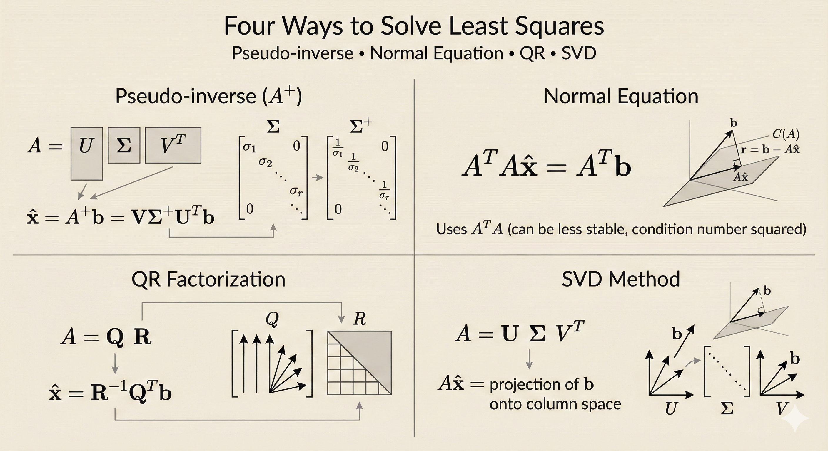
 Figure: Summary of four equivalent ways to solve least squares problems, all converging to the same optimal solution.
Key Insights
Multiple perspectives, same solution: The pseudo-inverse, normal equations, algebraic minimization, and geometric projection all lead to the same least-squares solution.
When \(A^T A\) is invertible: \(\hat{x} = (A^T A)^{-1}A^T b\) provides a closed-form solution.
Projection interpretation: Least squares finds the point in \(C(A)\) closest to \(b\)—this is the fundamental geometric insight.
Pseudo-inverse generalizes inversion: \(A^+ = V\Sigma^+ U^T\) extends matrix inversion to non-invertible matrices by inverting only non-zero singular values.