Goodfellow Deep Learning — Chapter 10.1: Unfold Computation Graph
Recurrent Model (RNN) is specified for sequence data processing. While CNN is specified for grid data (images), RNN is designed to process sequences \((x^{(1)},x^{(2)},...,x^{(t)})\).
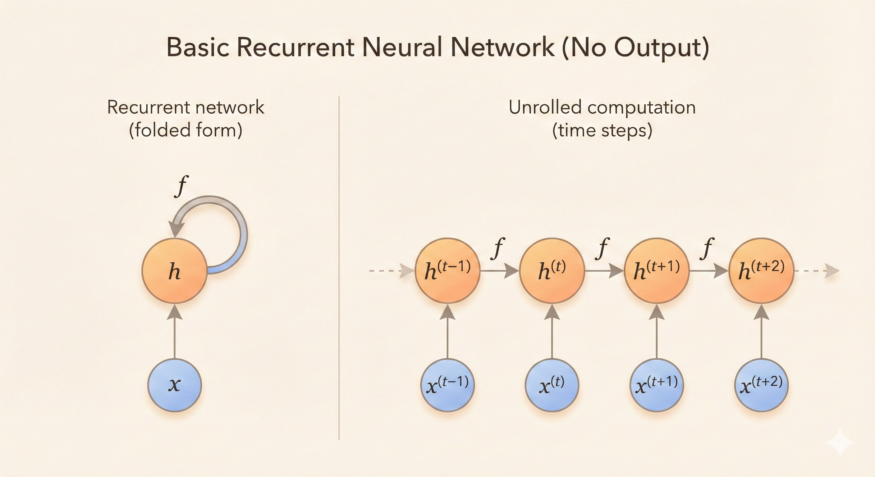
Parameter Sharing Through Unfolding
Unfolding the computation graph results in the parameters to be shared.
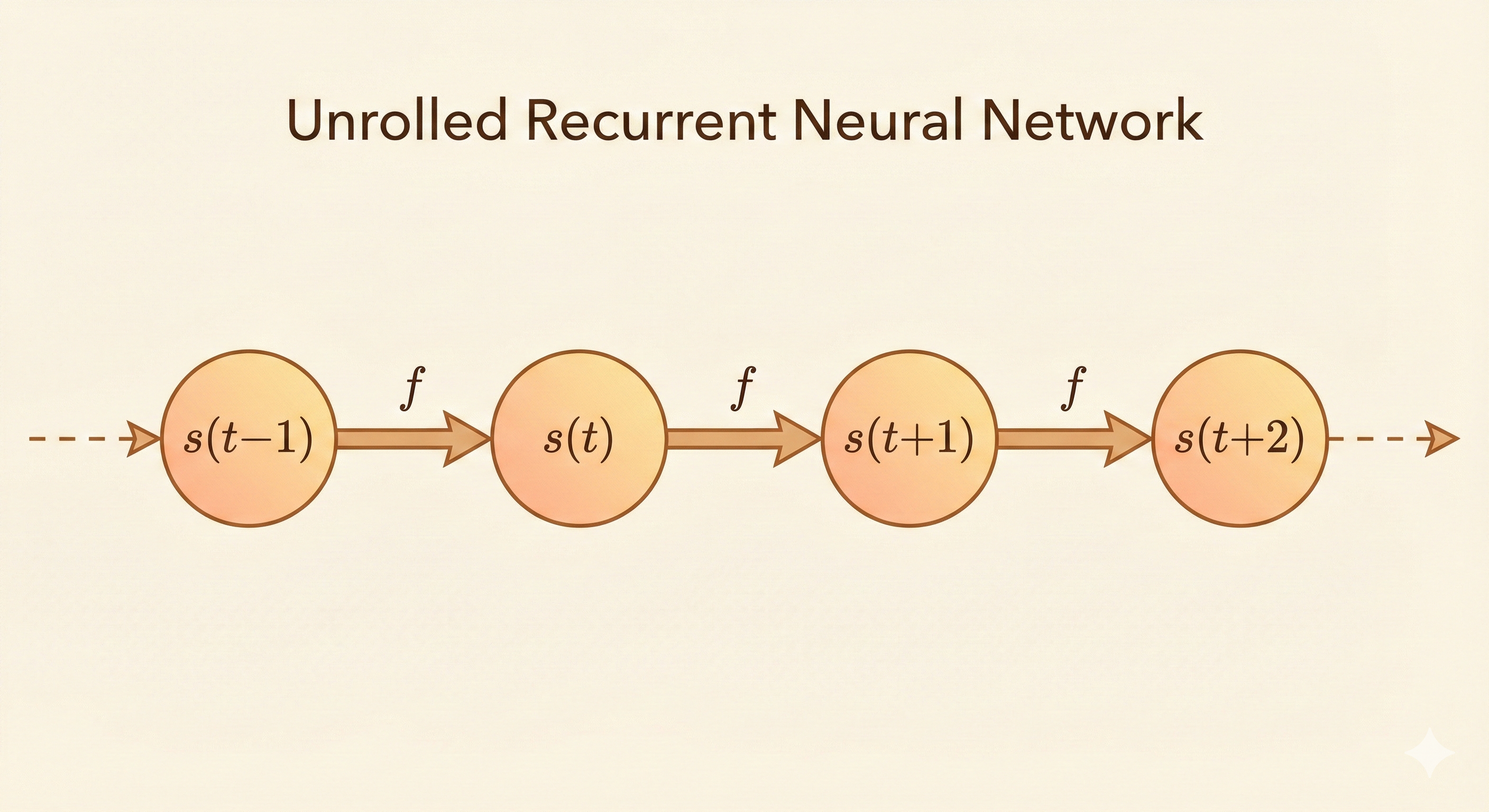
\[ s^{(t)}=f(s^{(t-1)};\theta) \tag{10.1} \]
where \(s^{(t)}\) is the system state.
The definition of \(s\) at time \(t\) depends on the moment of \(t-1\), so Equation 10.1 is recurrent.
\[ s^{(3)}=f(s^{(2)};\theta) \tag{10.2} \]
\[ s^{(3)}=f(f(s^{(1)};\theta);\theta) \tag{10.3} \]
Dynamic Systems with External Input
Another example is a dynamic system driven by external signal \(x^{(t)}\):
\[ s^{(t)}=f(s^{(t-1)}, x^{(t)};\theta) \tag{10.4} \]
A real case: Consider the sentence “I love deep learning”. When \(t=3\):
- \(s^{(t-1)}\) is the memory of “I love”
- \(x^{(t)}\) is the embedding of “deep”
The Function \(g^{(t)}\)
\(g^{(t)}\) is the composed transformation of the past \(t\) steps, not the loop itself:
\[ h^{(t)}=g^{(t)}(x^{(t)},x^{(t-1)},x^{(t-2)},...,x^{(2)},x^{(1)}) \tag{10.6} \]
This is equivalent to Equation 10.5.
The function \(g^{(t)}\) takes the entire history of inputs \((x^{(t)}, x^{(t-1)}, \ldots, x^{(1)})\) as its argument.
The unrolled recurrent architecture allows us to express \(g^{(t)}\) as a repeated composition of the same transition function \(f\).
Two Key Advantages
This formulation offers two key advantages:
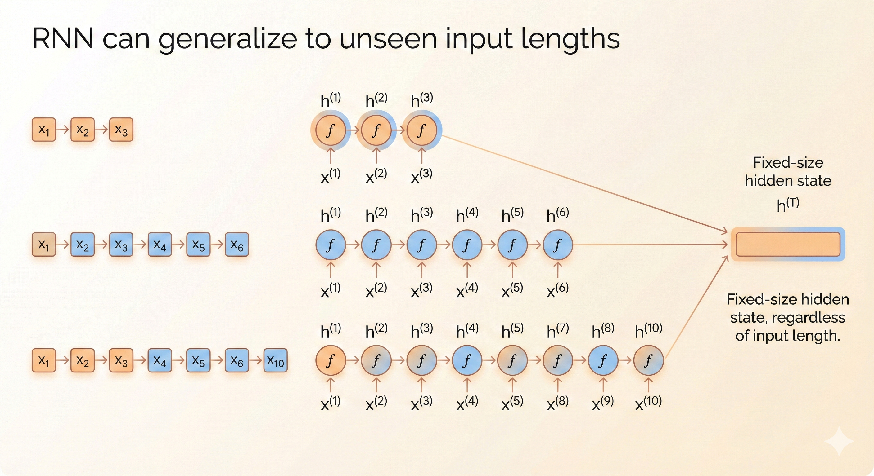
- Arbitrary input length: It allows inputs of arbitrary length to be mapped to a fixed-size hidden state
- Parameter sharing: It enables parameter sharing, since the same transition function \(f\) with the same parameters is reused at every time step
RNN models can also be generalized to unseen input lengths.
Key Insight
Unfolding computation graphs in RNNs enables parameter sharing across time steps. The same function \(f\) with parameters \(\theta\) is applied repeatedly, allowing the model to process sequences of any length while maintaining a fixed number of parameters. The hidden state \(h^{(t)}\) compresses the entire input history into a fixed-size representation, learning to retain only task-relevant information. This architecture generalizes naturally to unseen sequence lengths and enables three fundamental patterns: sequence-to-sequence (many-to-many), sequence-to-vector (many-to-one), and vector-to-sequence (one-to-many) mappings.