MIT 18.065: Lecture 18 - Counting Parameters in SVD, LU, QR, and Saddle Points
Counting parameters in matrix factorizations
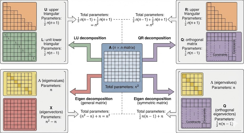
A general \(n\times n\) matrix has \(n^2\) free parameters. Each factorization splits those degrees of freedom across structured factors.
LU and QR
- \(L\) (unit lower‑triangular): \(\frac12 n(n-1)\) parameters (the diagonal is fixed to 1).
- \(U\) or \(R\) (upper‑triangular): \(\frac12 n(n+1)\) parameters.
Check: \[ \frac12 n(n-1)+\frac12 n(n+1)=n^2. \]
Eigenvalue decomposition
For a diagonalizable matrix \(A=X\Lambda X^{-1}\):
- \(\Lambda\) (diagonal): \(n\) eigenvalues.
- \(X\) (eigenvectors): each eigenvector has \(n\) components but scale is arbitrary, so each contributes \(n-1\) degrees of freedom. Total: \(n(n-1)=n^2-n\).
Check: \[ (n^2-n)+n = n^2. \]
Symmetric matrices
A symmetric matrix has \(\frac12 n(n+1)\) parameters. Its spectral form \(A=Q\Lambda Q^\top\) has:
- \(Q\) (orthogonal): \(\frac12 n(n-1)\)
- \(\Lambda\): \(n\)
Check: \[ \frac12 n(n-1)+n=\frac12 n(n+1). \]
SVD parameter counts
Let \(A\in\mathbb{R}^{m\times n}\) with rank \(r\).
Full‑rank case (\(m\le n\), rank \(r=m\))
\[ A=U\Sigma V^\top \]
- \(U\) (orthogonal \(m\times m\)): \(\frac12 m(m-1)\)
- \(\Sigma\): \(m\)
- \(V\) (only first \(m\) columns matter): \(m(n-1)-\frac12 m(m-1)\)
Check: \[ \frac12 m(m-1)+m+m(n-1)-\frac12 m(m-1)=mn. \]
General rank \(r\)
Use a reduced SVD with \(U\in\mathbb{R}^{m\times r}\), \(\Sigma\in\mathbb{R}^{r\times r}\), \(V\in\mathbb{R}^{r\times n}\).
Parameters:
- \(U\): \(mr-\frac12 r(r+1)\)
- \(\Sigma\): \(r\)
- \(V\): \(rn-\frac12 r(r+1)\)
Total: \[ mr+nr-r^2. \]
Saddle points
Consider the constrained quadratic problem \[ \begin{aligned} \text{minimize}&\quad \frac12 x^\top S x\\ \text{subject to}&\quad Ax=b. \end{aligned} \]
The Lagrangian is \[ L(x,\lambda)=\frac12 x^\top Sx+\lambda^\top(Ax-b). \]
Gradients: - \(\nabla_x L = Sx + A^\top\lambda\) - \(\nabla_\lambda L = Ax-b\)
The KKT system is \[ \begin{bmatrix} S & A^\top\\ A & 0 \end{bmatrix} \begin{bmatrix} x\\\lambda \end{bmatrix}= \begin{bmatrix} 0\\b \end{bmatrix}. \]
Because the block matrix is indefinite, the stationary point is a saddle in \((x,\lambda)\).
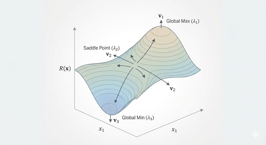
Saddle points from the Rayleigh quotient
\[ R(x)=\frac{x^\top S x}{x^\top x} \]
- Maximum at \(x=q_1\): \(R(x)=\lambda_1\).
- Minimum at \(x=q_n\): \(R(x)=\lambda_{\min}\).
Between them, the other critical points are saddles.
Takeaway. Parameter counting exposes the degrees of freedom hidden inside factorizations. It explains why \(LU\), \(QR\), eigendecomposition, and SVD all add up to the original matrix, and why saddle points naturally appear in constrained quadratic problems.