Goodfellow Deep Learning — Chapter 12.2: Image Preprocessing and Normalization
Deep Learning Book - Chapter 12.2 (page 444)
Computer vision tasks require careful preprocessing to improve model performance and training stability. This chapter covers normalization strategies and data augmentation techniques that enable deep learning models to learn robust visual representations.
Preprocessing
Preprocessing transforms raw image data into a form more suitable for learning algorithms. Two fundamental preprocessing techniques are normalization and data augmentation.
Normalization
Pixel value normalization rescales image intensities to a standard range, improving numerical stability and convergence during training.
Common normalization ranges: - [0, 1]: Divide pixel values by 255 (for 8-bit images) - [-1, 1]: Rescale to zero-centered range: (pixel / 127.5) - 1
Why normalization matters: - Ensures features are on similar scales - Prevents numerical instability in gradient computation - Improves optimization convergence - Reduces sensitivity to lighting variations
Data Augmentation
Data augmentation artificially expands the training set by applying transformations that preserve semantic labels while introducing realistic variations.
Common augmentation techniques: - Geometric transformations: Random rotations, translations, flips, crops - Color transformations: Brightness, contrast, saturation adjustments - Noise injection: Gaussian noise, blur, sharpening - Advanced techniques: Mixup, CutMix, AutoAugment
Benefits: - Reduces overfitting by increasing effective dataset size - Improves generalization to variations not seen during training - Acts as a regularization technique - Encodes invariances directly into training data
Data augmentation is a form of regularization that reduces generalization error without requiring additional labeled data. For image classification, simple transformations like random crops and horizontal flips can significantly improve test accuracy with minimal implementation cost.
Contrast Normalization
Contrast normalization aims to reduce sensitivity to lighting variations and enhance local image structures by normalizing pixel intensities across an image or within local neighborhoods.
Global Contrast Normalization (GCN)
Global Contrast Normalization subtracts the mean intensity and divides by the image’s standard deviation, ensuring each image has zero mean and unit variance.
Mathematical formulation:
For an image \(X\) with pixels \(X_{i,j,k}\) (where \(i,j\) index spatial location and \(k\) indexes color channel):
\[ X'_{i,j,k} = s \cdot \frac{X_{i,j,k} - \bar{X}}{\max(\epsilon, \sqrt{\lambda + \frac{1}{3rc}\sum_{i,j,k}(X_{i,j,k} - \bar{X})^2})} \]
where: - \(\bar{X}\) = mean intensity across all pixels and channels - \(s\) = target standard deviation (typically 1.0) - \(\epsilon\) = small constant to prevent division by zero (e.g., \(10^{-8}\)) - \(\lambda\) = regularization constant (e.g., 10) - \(r, c\) = image height and width - The denominator computes standard deviation with regularization
Interpretation: 1. Mean centering: \(X_{i,j,k} - \bar{X}\) removes the global mean 2. Variance normalization: Division by standard deviation rescales to unit variance 3. Regularization: \(\lambda\) prevents excessive amplification of near-constant images
Geometric interpretation:
GCN can be viewed as L2 norm normalization after mean centering, which projects each image onto a unit hypersphere in pixel space.
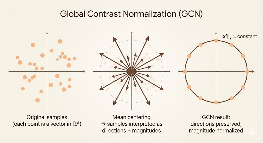
This geometric view reveals that GCN: - Normalizes all images to the same “magnitude” in pixel space - Removes global intensity scale while preserving contrast patterns - Makes the representation invariant to overall brightness changes
Local Contrast Normalization (LCN)
Local Contrast Normalization normalizes each pixel relative to its local neighborhood rather than the entire image.
Key differences from GCN: - Computes mean and standard deviation within a local window (e.g., 9×9 or 5×5) - Each pixel is normalized independently based on surrounding pixels - Enhances local structures like edges and textures
Advantages over GCN: 1. Local structure enhancement: Highlights edges and fine details 2. Robustness to spatially varying lighting: Different regions can have different brightness levels 3. Better biological plausibility: Mimics lateral inhibition in visual cortex 4. Preserves spatial detail: Prevents global statistics from dominating local patterns
Trade-offs: - More computationally expensive (requires convolution with local windows) - Can amplify noise in uniform regions - Requires careful choice of neighborhood size
Use GCN when: - Images have consistent global lighting - You want simple, fast preprocessing - Global intensity variations are the main concern
Use LCN when: - Images have spatially varying lighting - Local structure (edges, textures) is critical - Computational cost is acceptable
Contrast Normalization in Practice
Modern deep learning often relies on batch normalization and layer normalization during training rather than explicit preprocessing-based contrast normalization.
However, contrast normalization remains valuable for: - Preprocessing datasets with extreme lighting variations - Unsupervised feature learning (e.g., autoencoders, self-supervised methods) - Classical computer vision pipelines - Transfer learning from models trained on normalized data
Common practice: 1. Apply basic pixel normalization (e.g., scale to [0, 1]) 2. Use batch normalization within the network 3. Apply data augmentation (brightness, contrast adjustments) 4. Reserve GCN/LCN for cases where batch normalization is insufficient
Summary
Computer vision preprocessing requires careful consideration of:
- Pixel normalization: Rescale values to standard ranges ([0,1] or [-1,1])
- Data augmentation: Apply transformations to increase effective dataset size and encode invariances
- Global Contrast Normalization (GCN): Normalize entire image to zero mean and unit variance
- Local Contrast Normalization (LCN): Normalize each pixel relative to local neighborhood
Modern deep learning reduces reliance on explicit preprocessing through learned normalization layers, but understanding these techniques remains essential for handling challenging datasets and designing robust vision systems.