Lecture 14: Low Rank Changes and Their Inverse
Low-rank updates let us reuse an existing inverse instead of recomputing it from scratch. The Sherman–Morrison–Woodbury (SMW) identity is the workhorse: it turns an expensive \(n^3\) inverse into a small \(k^3\) inverse when the update has rank \(k\). Conceptually, \((A+UV^\top)^{-1}\) equals \(A^{-1}\) plus a low-rank correction, and computing that correction only requires solving a \(k\times k\) system.
Sherman–Morrison (rank-1)
For a rank-1 update \(I - uv^\top\), \[ (I-uv^\top)^{-1}=I+\frac{uv^\top}{1-v^\top u}. \] Here \(v^\top u\) is a scalar (a \(1\times 1\) matrix). A quick verification multiplies the two factors: \[ (I-uv^\top)\left(I+\frac{uv^\top}{1-v^\top u}\right)=I, \] so the formula holds as long as \(1-v^\top u\ne 0\).
Sherman–Morrison–Woodbury (rank-k)
For the general low-rank case, \[ (I_n-UV^\top)^{-1}=I_n+U(I_k-V^\top U)^{-1}V^\top, \] where \(U\in\mathbb{R}^{n\times k}\) and \(V^\top\in\mathbb{R}^{k\times n}\). When \(n\gg k\), this reduces complexity from \(n^3\) to \(k^3\).
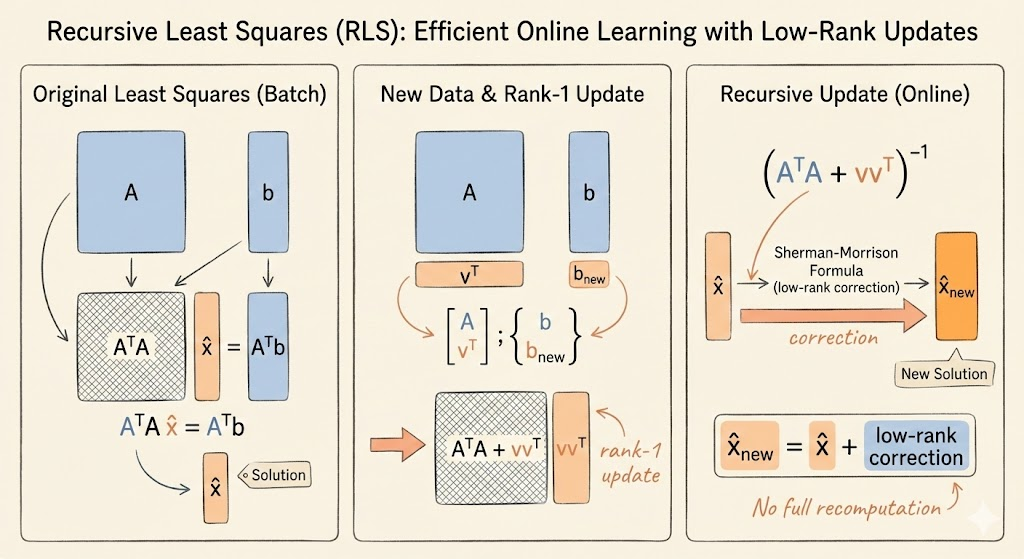
Use 1: Updating least squares
Suppose we solve \(Ax=b\) via normal equations \(A^\top A\hat{x}=A^\top b\). After adding one data point \([v,b_{new}]\), we get \[ (A^\top A+vv^\top)\hat{x}_{new}=A^\top b+v b_{new}. \] The update to \(A^\top A\) is rank-1, so we can reuse \((A^\top A)^{-1}\) and update the solution efficiently using SMW instead of recomputing the inverse. For instance, \[ (A^\top A+vv^\top)^{-1}=(A^\top A)^{-1}-\frac{(A^\top A)^{-1}vv^\top(A^\top A)^{-1}}{1+v^\top(A^\top A)^{-1}v}, \] which updates the inverse with only vector-matrix products. This is the core idea behind recursive least squares.
Kalman filtering generalizes this update idea to streaming measurements.
Use 2: Solving a shifted system
If \(Aw=b\) is already solved and we need \((A-uv^\top)x=b\), SMW gives a shortcut. Solve the two linear systems once: \[ Aw=b, \quad Az=u. \] This reuses the factorization of \(A\) without recomputing a full inverse. Then \[ (A-uv^\top)^{-1}=A^{-1}+\frac{A^{-1}u\,v^\top A^{-1}}{1-v^\top A^{-1}u}, \] so with \(w=A^{-1}b\) and \(z=A^{-1}u\), \[ (A-uv^\top)^{-1}b =w+\frac{z\,v^\top w}{1-v^\top z}. \]
SMW in full form
The general identity is \[ (A-UV^\top)^{-1}=A^{-1}+A^{-1}U(I-V^\top A^{-1}U)^{-1}V^\top A^{-1}. \]
It shows how to update inverses under low-rank changes without recomputing from scratch.
Key takeaways
- SMW replaces an \(n\times n\) inverse with a \(k\times k\) inverse plus low-rank corrections.
- The rank-1 update requires \(1-v^\top u\ne 0\); otherwise the update is singular.
- These formulas enable fast updates in streaming least squares and Kalman filtering.