Lecture 6: Singular Value Decomposition (SVD)

SVD vs Eigenvalue Decomposition

The Singular Value Decomposition extends the eigenvalue decomposition to any matrix (not just square or symmetric matrices).

Comparing the two factorizations:

• Eigenvalue decomposition (symmetric matrices): \(S=Q\Lambda Q^\top\)
  • Q: \(n \times n\) (orthogonal eigenvectors)
  • \(\Lambda\): \(n \times n\) (diagonal eigenvalues)
• SVD (any matrix): \(A=U\Sigma V^\top\)
  • U: \(m \times m\) (left singular vectors)
  • \(\Sigma\): \(m \times n\) (nonnegative singular values on the diagonal, usually ordered \(\sigma_1 \ge \sigma_2 \ge \dots\))
  • \(V^\top\): \(n \times n\) (right singular vectors)

Key relationships (square case):

\[ A^\top A=V \Sigma^\top \Sigma V^\top,\quad AA^\top=U \Sigma \Sigma^\top U^\top \]

---

Building SVD from Eigenvectors

For a rectangular matrix A of rank r, the singular vectors satisfy:

\[ Av_r=\sigma_r u_r\\ Av_{r+1}=0 \]

Stacking these relationships for all r singular vectors:

\[ A[v_1,\dots,v_r]=[u_1\dots u_r]\begin{bmatrix}\sigma_1&&\\&\ddots&\\&&\sigma_r\end{bmatrix}\\ AV=U\Sigma\\ A=U\Sigma V^\top \]

---

Computing \(U\), \(\Sigma\), and \(V\)

Computing V (right singular vectors)

\[ A^\top A=V\Sigma^\top \Sigma V^\top \]

• V: eigenvectors of \(A^\top A\)
• \(\Sigma^2\): eigenvalues of \(A^\top A\)

Computing U (left singular vectors)

\[ AA^\top=U\Sigma V^\top V \Sigma ^\top U^\top=U \Sigma \Sigma^\top U^\top \]

• U: eigenvectors of \(AA^\top\)
• \(\Sigma^2\): eigenvalues of \(AA^\top\)

Orthogonality of U induced by V

The left singular vectors U are automatically orthogonal because V is orthogonal:

\[ u_1=\frac{Av_1}{\sigma_1},\quad u_r=\frac{Av_r}{\sigma_r}\\ u_1^\top u_r=\frac{v_1^\top A^\top A v_r}{\sigma_1 \sigma_r}=\frac{v_1^\top \sigma_r^2 v_r}{\sigma_1 \sigma_r}=\frac{\sigma_r v_1^\top v_r}{\sigma_1}=0 \]

Since \(v_1^\top v_r = 0\) (orthogonal eigenvectors), the left singular vectors are orthogonal.

---

Repeated Eigenvalues

When eigenvalues repeat, the eigenvectors span a subspace rather than being unique.

Example:

\[ \begin{bmatrix}1&0&0\\0&1&0\\0&0&5\end{bmatrix}\begin{bmatrix}x\\y\\0\end{bmatrix}=\begin{bmatrix}x\\y\\0\end{bmatrix} \]

For \(\lambda_1=\lambda_2=1\), the entire xy-plane is the eigenspace—any vector in that plane is an eigenvector.

---

Geometric Interpretation

SVD decomposes any linear transformation into three steps: rotate, scale, rotate.

\[ Ax=U \Sigma V^\top x \]

1. \(x'=V^\top x\): Rotate x by \(V^\top\) (change of basis to V coordinates)
2. \(x''=\Sigma x'\): Scale along each singular direction by \(\sigma_i\)
3. \(Ax=Ux''\): Rotate result by U to final position

2D Example:

\[ A=\begin{bmatrix}1&2\\-2&1\end{bmatrix},\quad x=\begin{bmatrix}1\\1\end{bmatrix} \]

SVD geometric transformation

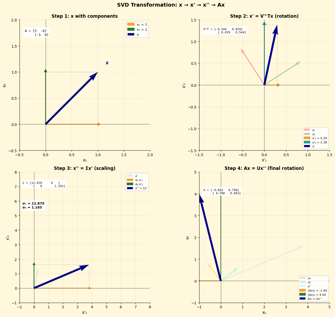
The transformation rotates, stretches by \(\sigma_1\) and \(\sigma_2\), then rotates again.

---

Singular Values, Determinants, and Eigenvalues

Since both U and V are orthogonal matrices with determinant ±1:

\[ \det A=\prod_{i=1}^r \sigma_i \]

For square matrices:

\[ \det A=\prod_{i=1}^r \sigma_i=\prod_{i=1}^n \lambda_i \]

Example:

\[ A=\begin{bmatrix}3&4\\0&5\end{bmatrix} \]

• Singular values (sorted): \(\sigma_1\approx 6.708,\ \sigma_2\approx 2.236\)
• Eigenvalues: \(\lambda_1=3,\ \lambda_2=5\)
• Magnitudes of eigenvalues are bounded by the largest singular value: \(|\lambda_i|\le \sigma_1\); there is no ordering between individual \(\lambda_i\) and \(\sigma_i\) unless \(A\) is normal.
• Product: \(\sigma_1 \sigma_2=|\det A|=15\), and \(\lambda_1\lambda_2=\det A=15\)

Special case: When A is symmetric, singular values equal absolute values of eigenvalues.

---

Polar Decomposition

Every matrix can be written as the product of a symmetric positive semidefinite matrix and an orthogonal matrix:

\[ A=SQ \]

By inserting \(U^\top U=I\):

\[ A=U\Sigma V^\top = (U\Sigma U^\top)( U V^\top) \]

• \(UV^\top\) is orthogonal (product of orthogonal matrices)
• \(U\Sigma U^\top\) is symmetric positive semidefinite

This is analogous to writing a complex number in polar form: \(z = r e^{i\theta}\) (magnitude × rotation).

---

Exercises

Exercise 1

Find \(\sigma\)’s, \(u\)’s and \(v\)’s in the SVD for \(A=\begin{bmatrix}3&4\\0&5\end{bmatrix}\).

Solution:

1. Compute \(A^\top A\) and \(AA^\top\): \[ A^\top A=\begin{bmatrix}9&12\\12&41\end{bmatrix},\quad AA^\top=\begin{bmatrix}25&20\\20&25\end{bmatrix} \]

2. Find singular values from eigenvalues of \(AA^\top\):

   • Trace: \(\sigma_1^2+\sigma_2^2=50\)
   • Determinant: \(\sigma_1^2 \cdot \sigma_2^2=125\)
   • Solving: \(\sigma_1=\sqrt{5}\), \(\sigma_2=\sqrt{45}\)

3. Right singular vectors (eigenvectors of \(A^\top A\)):

   • \(A^\top A- 5I=\begin{bmatrix}4&12\\12&36\end{bmatrix}\) has nullspace \([-3,1]\)
     • Normalized: \(v_1=\frac{1}{\sqrt{10}}\begin{bmatrix}-3\\1\end{bmatrix}\)
   • \(A^\top A - 45I=\begin{bmatrix}-36&12\\12&-4\end{bmatrix}\) has nullspace \([1,3]\)
     • Normalized: \(v_2=\frac{1}{\sqrt{10}}\begin{bmatrix}1\\3\end{bmatrix}\)

4. Left singular vectors (eigenvectors of \(AA^\top\)):

   • \(AA^\top - 5I=\begin{bmatrix}20&20\\20&20\end{bmatrix}\) has nullspace \([1,-1]\)
     • Normalized: \(u_1=\frac{1}{\sqrt{2}}\begin{bmatrix}1\\-1\end{bmatrix}\)
   • \(AA^\top - 45I=\begin{bmatrix}-20&20\\20&-20\end{bmatrix}\) has nullspace \([1,1]\)
     • Normalized: \(u_2=\frac{1}{\sqrt{2}}\begin{bmatrix}1\\1\end{bmatrix}\)

---

Exercise 2

A symmetric matrix \(S = S^\top\) has orthonormal eigenvectors \(v_1\) to \(v_n\). Then any vector x can be written as \(x = c_1v_1 + \cdots + c_nv_n\). Explain these two formulas:

(a) \(x^\top x=c_1^2+\dots+c_n^2\)

Solution:

\[ x^\top x=(c_1v_1)^\top c_1v_1+\dots+(c_nv_n)^\top c_n v_n=c_1^2v_1^\top v_1+\dots+c_n^2v_n^\top v_n \]

Because \(v_1,\dots, v_n\) are orthonormal, \(v_i^\top v_i=1\) for all i, so:

\[ x^\top x=c_1^2+\dots+c_n^2 \]

This is Parseval’s identity: the norm squared equals the sum of squared coefficients.

(b) \(x^\top S x=\lambda_1 c_1^2+\dots+\lambda_n c_n^2\)

Solution:

\[ Sx=S(c_1v_1+\dots+c_nv_n)=c_1Sv_1+\dots+c_nSv_n=c_1\lambda_1v_1+\dots+c_n\lambda_nv_n \]

\[ x^\top Sx=c_1^2\lambda_1 v_1^\top v_1+\dots+c_n^2\lambda_n v_n^\top v_n=\lambda_1c_1^2+\dots+\lambda_n c_n^2 \]

This shows the quadratic form \(x^\top Sx\) is a weighted sum of squared coefficients, weighted by eigenvalues. This connects to optimization: minimizing \(x^\top Sx\) favors directions with small eigenvalues.