Goodfellow Deep Learning — Chapter 16: Structured Probabilistic Models for Deep Learning
Source: Deep Learning Book (Ian Goodfellow, Yoshua Bengio, Aaron Courville) - Chapter 16
Structured probabilistic models represent complex probability distributions by explicitly modeling dependencies among random variables using graph structures.
The graph encodes which variables interact directly, enabling the factorization of high-dimensional distributions into simpler components.
This structure provides a principled way to manage complexity, design large-scale probabilistic models, and reason about learning and inference, including in settings where neural networks parameterize parts of the model.
The challenge of unstructured modeling
Modeling complex, high-dimensional data such as images requires estimating the full joint distribution p(x) over a large number of random variables.
Tasks like density estimation, denoising, missing-value imputation, and sampling all rely on having a coherent model of this joint distribution, since even a single unlikely component should reduce the probability of the entire configuration.
However, directly representing \(p(x)\) in a naive, table-based manner is infeasible.
For a random vector x with n discrete variables, each taking k possible values, such an approach requires \(k^n\) parameters.
Even in the simplest case of binary variables, this number grows astronomically.
For example, a small \(32 \times 32\) RGB image contains thousands of variables, leading to more possible configurations than can be meaningfully stored, learned, or enumerated.
This exponential complexity makes naive joint modeling impossible along several dimensions:
it exceeds memory limits, requires an unrealistic amount of training data to estimate parameters reliably, and renders inference and sampling computationally intractable.
The root cause is that the table-based approach implicitly assumes arbitrary interactions among all subsets of variables, treating every dependency as equally important.
Use Graphs to Describe Model Structure
Structured probabilistic models use graph to represent interactions between random variables.
- Each node represents a random variable
- Each edge represents a direct interaction.
Directed Models
The direction of the arrow indicates the which variable’s probability distribution depends on the other’s.
Example:
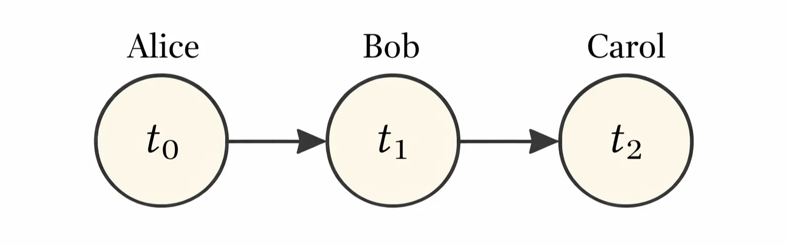
In the relay race example, Bob’s finishing time depends directly on Alice’s finishing time because Bob cannot start running until Alice finishes, while Carol’s finishing time depends directly on Bob’s finishing time and only indirectly on Alice’s, since Alice influences Carol solely through Bob.
A directed graph model defined on variable \(x\) is defined by a directed asyclic graph \(\mathcal{G}\):
- \(Pa_{\mathcal{G}}(x_i)\), the parents of \(x_i\) in \(\mathcal{G}\)
- \(x_i\), the ith component of x
\[ p(x)=\prod_ip(x_i| Pa_\mathcal{G}(x_i)) \]
In our relay race example, this is
\[ p(t_0,t_1,t_2)=p(t_0)p(t_1|t_0)p(t_2|t_1) \]
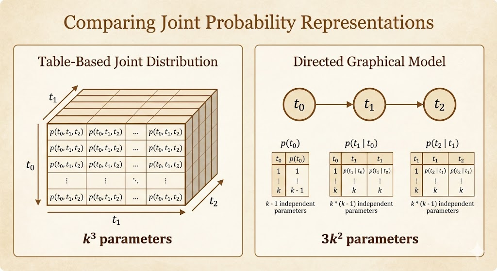
In a table-based approach, modeling the full joint distribution requires storing a parameter for every possible configuration of all variables, leading to exponential growth in storage. In contrast, a directed graphical model exploits conditional independence by factorizing the joint distribution into local conditional probabilities, so parameter storage scales with the number of variables and the size of their parent sets rather than with the full state space.
Undirected Models
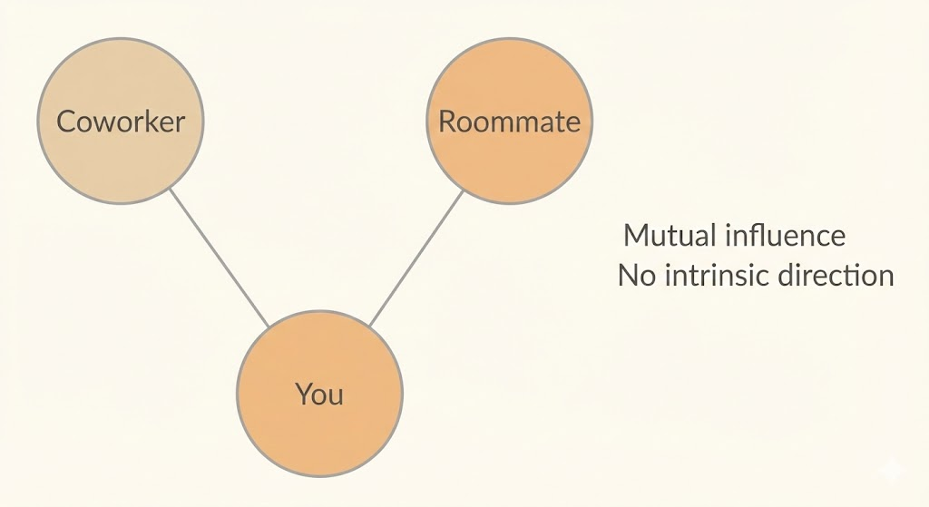
Undirected models, also known as Markov Random Fields (MRFs) or Markov networks, represent structured probabilistic relationships using graphs whose edges have no direction. Unlike directed models, they do not encode causal or temporal order. Instead, an undirected edge indicates that two random variables interact directly and symmetrically.
This representation is useful when the dependencies among variables have no clear intrinsic direction, or when influences operate mutually or cyclically. In such cases, forcing a directed (causal) interpretation would be unnatural or misleading. Undirected models allow us to capture patterns of mutual dependence without committing to a specific generative story.
As a result, undirected models are especially appropriate for systems where interactions are best understood as constraints or correlations rather than cause-and-effect processes.
Example
Consider modeling whether you, your coworker, and your roommate are sick, where infections may spread through close contact. Because these interactions have no clear intrinsic direction and can plausibly occur in either way, the dependencies are more naturally represented using an undirected model rather than a directed one.
\[ \tilde{p}(x)=\prod_{\mathcal{c}\in \mathcal{G}}\phi(\mathcal{C}) \]
- \(\mathcal{C}\): A clique is a subset of nodes in an undirected graph in which every pair of nodes is connected by an edge.
- x: denotes a joint assignment of all random variables in the graph.
- \(\phi(\mathcal{C})\): is a nonnegative potential function measuring the compatibility of variables in clique C.
- \(\tilde{p}(x)\): the unnormalized probability
| h_y = 0 | h_y = 1 | |
|---|---|---|
| h_c = 0 | 2 | 1 |
| h_c = 1 | 1 | 10 |
A state of 1 indicates good health, while a state of 0 indicates poor health (having been infected with a cold). Both individuals are usually healthy, so the state in which both h_c and h_y are 1 has the highest affinity. The state in which exactly one of them is sick has the lowest affinity, since this is a rare configuration. The state in which both are sick, corresponding to one individual infecting the other, has higher affinity than mixed states, though it is still less common than the state in which both are healthy.
The Partition Function
To obtain a valid probability distribution, we must do normalization
\[ p(x)=\frac{1}{Z}\tilde{p}(x) \]
where Z is the probability distribution integration or summing
\[ Z=\int \tilde{p}(x) d(x) \]
Unlike directed models, undirected models are defined by potentials rather than probabilities, and careless choices of potentials or variable domains may lead to models that cannot be normalized and therefore do not define valid probability distributions.
Energy-Based Models
A convenient way is to enforce the potential to use an energy-based model,
\[ \tilde{p}(x)=\exp(-E(x)) \]
where \(E(x)\) is known as energy-based model.
Any distribution of the form given by this equation is also called Boltzmann distribution.
Because \(\exp (a) \exp (b)=\exp(a+b)\), we found the clique correspond to the terms of the energy function.
\[ \tilde p(x) = \prod_{C \in \mathcal C} \phi_C(x_C)= \tilde p(x) = \exp\!\left(-\sum_C E_C(x_C)\right) \]
Separation
Graphical models encode direct interactions through edges, but indirect interactions may arise through paths in the graph.
- Conditional independence questions can be answered without computing probabilities, using only the graph structure.
- In undirected graphical models, conditional independence is determined by separation:
- Two sets of variables A and B are conditionally independent given a set S if all paths between A and B pass through at least one observed variable in S.
- Paths containing only unobserved variables are active, while paths containing any observed variable are inactive.
- Observed variables are often represented by shaded nodes in the graph to visually indicate which paths are blocked.
- In directed graphical models, a related concept called d-separation is used:
- D-separation generalizes separation by accounting for the direction of edges.
- Two variables are conditionally independent if there is no active path between them according to the d-separation rules.
- Separation and d-separation provide a graphical criterion for conditional independence, forming the basis for reasoning, inference, and model design in probabilistic graphical models.
Converting
- Directed and undirected graphical models encode conditional independencies in different ways and are not generally equivalent.
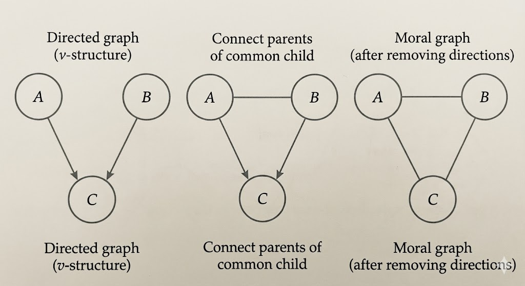
- Converting a directed graph to an undirected graph requires moralization, which connects parents of a common child and removes edge directions.
- Moralization typically introduces additional edges and therefore removes some conditional independence relationships.
- Undirected graphs containing cycles of length greater than three cannot be converted directly into directed acyclic graphs.
- Such graphs must first be triangulated by adding chords, producing a chordal (triangulated) graph.
- Adding chords introduces new dependencies and reduces the set of independencies represented by the graph.
- After triangulation, edges can be assigned directions while avoiding directed cycles, often by imposing an ordering on variables.
- In general, converting between directed and undirected models requires adding edges and results in a loss of independence information.
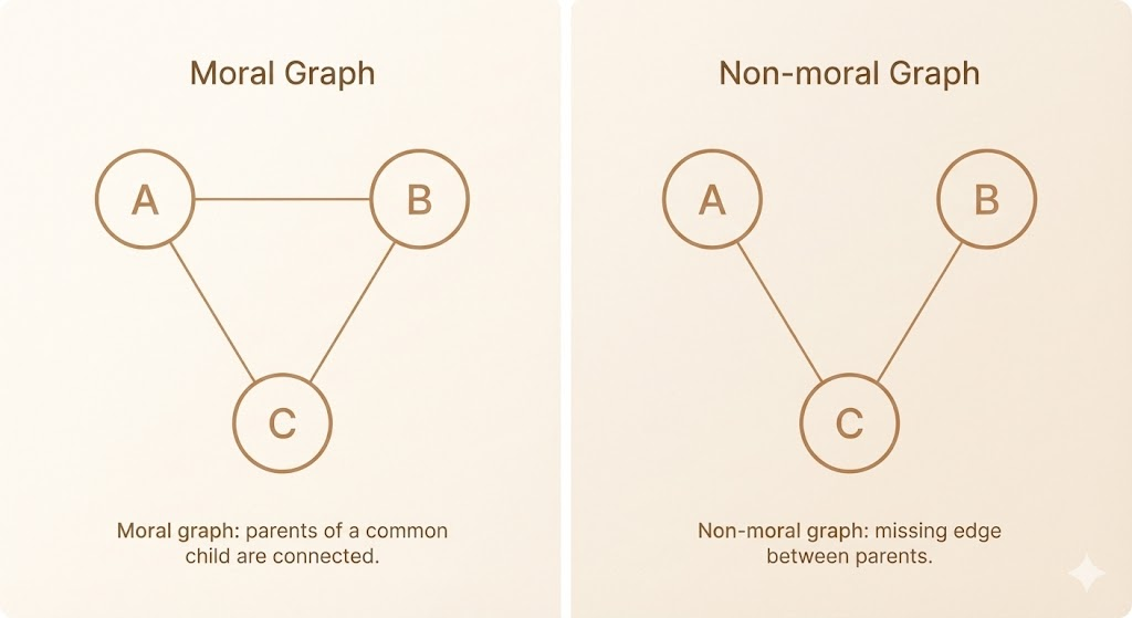
Moral Graph
- A moral graph is an undirected graph obtained from a directed acyclic graph by a process called moralization.
- Moralization consists of connecting all parents of each node and then removing the directions of all edges.
- This process ensures that dependencies implied by shared children in the directed model are preserved in the undirected representation.
- Moral graphs typically contain additional edges compared to the original directed graph.
- As a result, some conditional independencies present in the directed model may be lost.
- Moralization is generally necessary when converting a directed graphical model into an undirected one, but the conversion is not lossless in general.
Moralization
Factor Model
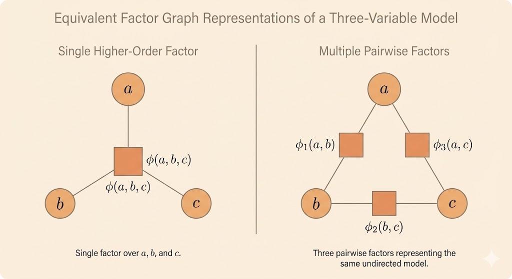
- Factor graphs provide an explicit representation of how a joint distribution factorizes into local functions.
- They resolve an ambiguity in undirected graphs, where a clique does not uniquely specify whether it corresponds to a single high-order factor or multiple lower-order factors.
- A factor graph is a bipartite graph consisting of two types of nodes: variable nodes and factor nodes.
- Variable nodes represent random variables, while factor nodes represent unnormalized factors (or potentials).
- An edge connects a variable node to a factor node if and only if the variable appears in that factor.
- Different factor graphs can represent the same joint distribution while using different factorizations.
- Although such factorizations are probabilistically equivalent, they can have very different computational properties for inference.
- Factor graphs provide a natural foundation for message-passing algorithms such as belief propagation.
- By making the factorization structure explicit, factor graphs improve clarity and flexibility in the design of inference algorithms.
Sampling
- Graphical models provide a structured way to generate samples from a joint probability distribution.
- Directed graphical models allow efficient sampling via ancestral sampling.
- Ancestral sampling requires ordering variables in a topological order such that parents are sampled before their children.
- Sampling proceeds sequentially by drawing each variable from its conditional distribution given its parents.
- Ancestral sampling is fast and simple when local conditional distributions are easy to sample from.
- Ancestral sampling applies only to directed models and does not naturally support conditional sampling given arbitrary observed variables.
- Conditional sampling in directed models may require sampling from posterior distributions, which are often not explicitly parameterized and can be computationally expensive.
- Undirected graphical models do not admit ancestral sampling due to cyclic dependencies among variables.
- Sampling from undirected models generally requires iterative procedures rather than a single forward pass.
- The most basic sampling method for undirected models is Gibbs sampling.
- Gibbs sampling updates one variable at a time by sampling from its conditional distribution given all other variables.
- Due to the separation properties of graphical models, each update only needs to condition on the variable’s neighbors.
- A single sweep over all variables does not produce an independent sample from the target distribution.
- Repeated iterations are required, and the sampling process converges asymptotically to the correct distribution.
- Determining when Gibbs sampling has converged can be difficult.
- Sampling methods for undirected models are more computationally expensive and are treated as an advanced topic.
Structured Probabilistic Models: Motivation, Challenges, and the Deep Learning Perspective
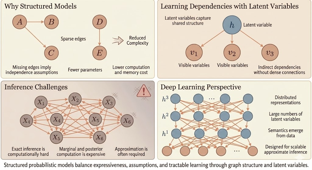
Structured probabilistic models are introduced to make complex probability distributions tractable by explicitly encoding assumptions about how variables interact. Instead of modeling all variables as fully connected, structure is imposed through sparse graphs, where missing edges represent conditional independence assumptions. This dramatically reduces the number of parameters, lowers computational and memory costs, and makes learning and reasoning feasible in high-dimensional settings.
However, real-world data often exhibits strong dependencies among observed variables. Directly modeling all such dependencies would require dense graphs with large cliques, leading to exponential growth in parameters and data requirements. To resolve this, latent variables are introduced. Latent variables capture shared, underlying structure and allow observed variables to interact indirectly, enabling rich dependencies without dense direct connections. In this way, complex correlations among visible variables can be explained efficiently through a smaller number of hidden causes.
Despite these modeling advantages, inference remains a central challenge. Many important probabilistic queries—such as computing marginals or posterior distributions over latent variables—are computationally intractable in general graphical models. Exact inference is often prohibitively expensive, even when the model structure is carefully designed. As a result, approximate inference methods become necessary, trading exactness for scalability.
The deep learning perspective embraces this trade-off explicitly. Rather than designing models to preserve exact inference, deep learning focuses on scalable approximate inference using distributed representations and large numbers of latent variables. Deep models rely on simple, repetitive connectivity patterns and parameter sharing, allowing efficient computation on modern hardware. Semantics are not hard-coded into individual latent variables; instead, meaningful structure emerges from data through learning. Approximate inference techniques such as variational inference or sampling are treated as integral components of the model design, rather than as afterthoughts.