Gilbert Strang’s Calculus: Highlights
“Calculus is about pairs of functions.” — Gilbert Strang
Reference: Highlights of Calculus (MIT OCW)
Derivatives: rates of change
Calculus connects a function to its rate of change. The derivative tells us how fast \(y\) changes when \(x\) changes.
Basic rules
- Constant: \(\dfrac{d}{dx}(u+c)=\dfrac{du}{dx}\)
- Sum: \(\dfrac{d}{dx}(u+v)=\dfrac{du}{dx}+\dfrac{dv}{dx}\)
- Product: \(\dfrac{d}{dx}(uv)=u\,\dfrac{dv}{dx}+v\,\dfrac{du}{dx}\)
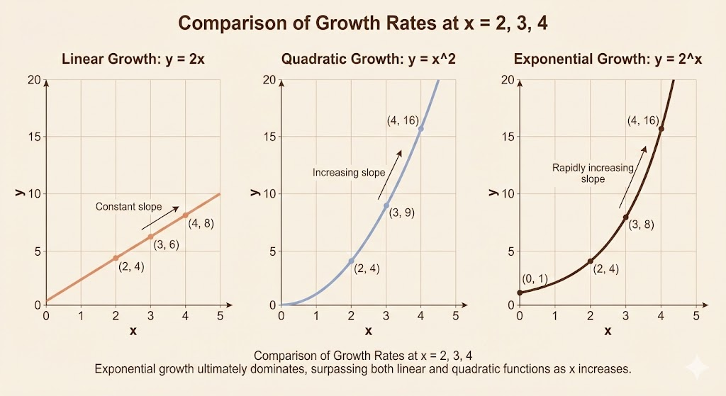
Three example functions
- Linear: \(y=2x\) (constant growth)
- Quadratic: \(y=x^2\) (growth increases with \(x\))
- Exponential: \(y=2^x\) (growth increases explosively)
These have very different growth rates, even though they all increase.
Calculating change
There are two perspectives on change:
- Limits: \(\dfrac{\Delta y}{\Delta x}\), then take \(\Delta x\to 0\)
- Rules: start from known derivatives and build new ones
For a linear combination, \[ \frac{d}{dx}(C_1y_1+C_2y_2)=C_1\frac{dy_1}{dx}+C_2\frac{dy_2}{dx}. \]
Example: if \(y=x^2-1\), then \(\dfrac{dy}{dx}=2x\).
Slope and the tangent line
The average slope between two points is \[ \frac{y_2-y_1}{x_2-x_1}=\frac{\Delta y}{\Delta x}. \] The instantaneous slope is the limit as \(\Delta x\to 0\).
For \(y=x^2\), \[ \frac{\Delta y}{\Delta x}= \frac{(x+\Delta x)^2-x^2}{\Delta x}=2x+\Delta x \quad\Rightarrow\quad \frac{dy}{dx}=2x. \]
This produces the linear approximation near \(x_0\): \[ y\approx y_0+\frac{dy}{dx}(x_0)(x-x_0). \]
Second derivative
The second derivative is the slope of the slope. If \(y=x^2\), then \(\dfrac{dy}{dx}=2x\) and \(\dfrac{d^2y}{dx^2}=2\). It tells us whether the function is speeding up or slowing down.
Power rule
For \(y=x^n\), \[ \frac{dy}{dx}=n x^{n-1}. \]
Examples: - \(y=x^2 \Rightarrow \dfrac{dy}{dx}=2x\) - \(y=x^3 \Rightarrow \dfrac{dy}{dx}=3x^2\) - \(y=x^4 \Rightarrow \dfrac{dy}{dx}=4x^3\)
Sketch of proof (induction): Assume \(\dfrac{d}{dx}x^n=nx^{n-1}\). Then \[ \frac{d}{dx}(x\cdot x^n)=1\cdot x^n + x\cdot (n x^{n-1})=(n+1)x^n. \]
Exponential function
The exponential function \(y=e^x\) solves \[ \frac{dy}{dx}=y. \] It equals its own slope.
Series expansion: \[ e^1=e=1+1+\frac{1}{2}+\frac{1}{6}+\frac{1}{24}+\dots \]
Key rules: - \(e^{x_1}e^{x_2}=e^{x_1+x_2}\) - \((e^x)^n=e^{xn}\)
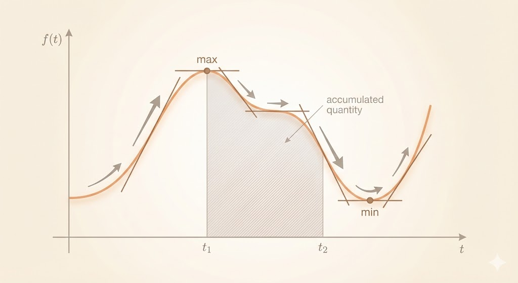
Maxima and minima
To find extrema of \(y=f(x)\), solve \[ \frac{dy}{dx}=0 \] for critical points. The second derivative distinguishes max vs. min.
Integrals: accumulation
If the derivative is speed, the integral is distance. If the derivative is a rate, the integral is the total effect.
The graph already contains the integral: the area under the curve measures accumulation.
Graphs as reasoning tools
In Highlights of Calculus, graphs are not for decoration—they are reasoning tools. Slope reveals the first derivative, concavity reveals the second derivative, and extrema and inflection points become visible directly from shape.
Takeaway. Calculus links pairs: a function and its derivative, or a rate and its accumulation. These connections let us read change from shape and compute global behavior from local rules.