EE 364A (Convex Optimization): Chapter 4.5 - Geometric Programming
Geometric Programming
Geometric programming (GP) is a class of problems built from monomials and posynomials over positive variables. With a logarithmic change of variables, a GP becomes a convex optimization problem, so it can be solved efficiently and globally.
Monomial functions
A monomial has the form \[ f(x)=c x_1^{a_1}x_2^{a_2}\dots x_n^{a_n},\quad \mathrm{dom}\,f=\mathbb{R}_{++}^n. \]
- \(c>0\).
- In algebraic monomials, \(c\) can be any real number.
- In GP, \(c\) must be positive so we can write \(c=e^{\log c}\).
- \(a_i\in\mathbb{R}\).
Posynomials
A posynomial is a sum of monomials: \[ f(x)=\sum_{k=1}^K c_k x_1^{a_{1k}}x_2^{a_{2k}}\dots x_n^{a_{nk}},\quad \mathrm{dom}\,f=\mathbb{R}_{++}^n. \]
Standard GP form
A geometric program is \[ \begin{aligned} \text{minimize} &\quad f_0(x) \\ \text{subject to} &\quad f_i(x)\le 1,\quad i=1,\dots,m \\ &\quad h_i(x)=1,\quad i=1,\dots,p, \end{aligned} \] where - \(f_0,f_i\) are posynomials, - \(h_i\) are monomials, - the domain is \(\mathbb{R}_{++}^n\).
GP in convex form
GP is not a standard convex program in \(x\), but it becomes convex after a log change of variables.
For a monomial \[ f(x)=c x_1^{a_1}\dots x_n^{a_n}, \] define - \(y_i=\log x_i\) so \(x_i=e^{y_i}\), - \(b=\log c\) so \(c=e^b\). Then \[ f(x)=e^{a^\top y+b}. \]
For a posynomial \[ f(x)=\sum_{k=1}^K c_k x_1^{a_{1k}}\dots x_n^{a_{nk}}, \] we get \[ f(x)=\sum_{k=1}^K e^{a_k^\top y+b_k}. \]
So the GP becomes \[ \begin{aligned} \text{minimize} &\quad \sum_{k=1}^{K_0} e^{a_{0k}^\top y+b_{0k}} \\ \text{subject to} &\quad \sum_{k=1}^{K_i} e^{a_{ik}^\top y+b_{ik}} \le 1,\quad i=1,\dots,m \\ &\quad e^{g_i^\top y+h_i}=1,\quad i=1,\dots,p. \end{aligned} \] The monomial equality constraint is equivalent to the affine constraint \[ g_i^\top y+h_i=0. \]
It is also common to take logs of the posynomial constraints and objective (monotone transformation): \[ \tilde f_i(y)=\log\Big(\sum_{k=1}^{K_i} e^{a_{ik}^\top y+b_{ik}}\Big),\quad i=0,\dots,m. \] Then the convex form is \[ \begin{aligned} \text{minimize} &\quad \tilde f_0(y) \\ \text{subject to} &\quad \tilde f_i(y)\le 0,\quad i=1,\dots,m \\ &\quad g_i^\top y+h_i=0,\quad i=1,\dots,p. \end{aligned} \] Here \(\tilde f_i\) are log-sum-exp functions (convex), and the equality constraints are affine, so the problem is convex.
Examples
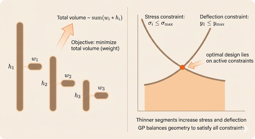
Cantilever beam design
We design a cantilever beam with a vertical load \(F\) applied at the free end. The beam is split into \(N\) equal-length segments. Segment \(i\) has a rectangular cross section with width \(w_i\) and height \(h_i\).
The goal is to minimize total volume while respecting geometry and mechanics: \[ \min \sum_{i=1}^N w_i h_i. \]
Subject to: - Geometric bounds: \[ w_{\min} \le w_i \le w_{\max},\quad h_{\min} \le h_i \le h_{\max}. \] - Aspect ratio constraints: \[ S_{\min} \le \frac{h_i}{w_i} \le S_{\max}. \] - Stress constraints: \[ \sigma_i = \frac{6 i F}{w_i h_i^2} \le \sigma_{\max}. \] - Deflection constraint: \[ y_1 \le y_{\max}. \]
The deflections \(y_i\) and slopes \(v_i\) follow beam-recursion relations with boundary conditions \(v_{N+1}=y_{N+1}=0\).
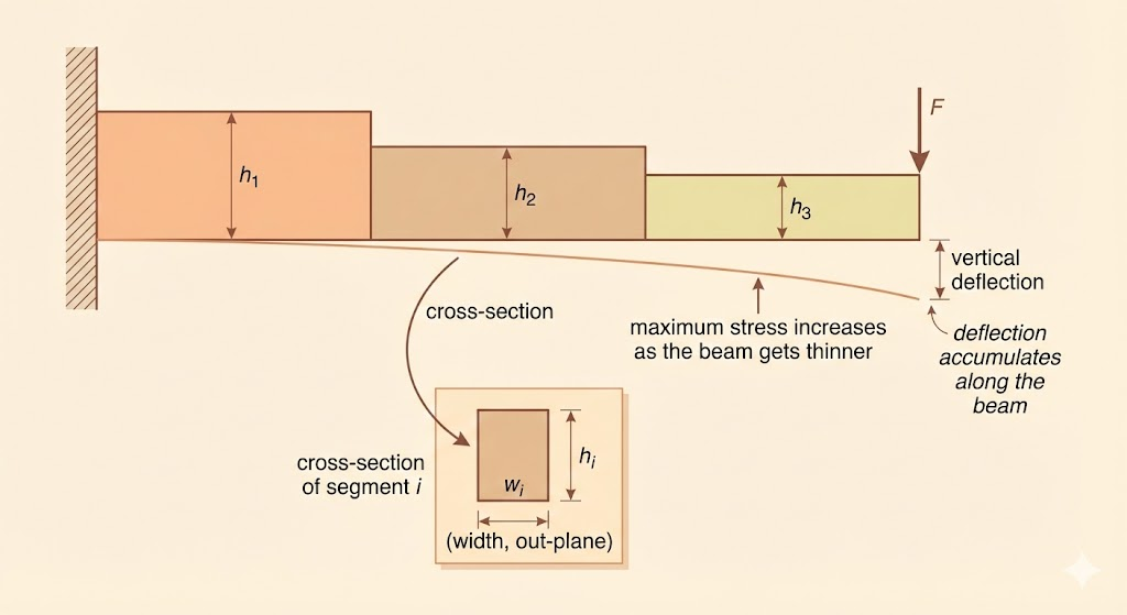
Why this is a GP - Each term \(w_i h_i\) is a monomial, so the volume is a posynomial. - Geometric bounds and aspect ratio constraints can be written as monomial inequalities. - Stress constraints take the monomial form \(c\,w_i^{-1}h_i^{-2}\le\sigma_{\max}\). - The recursive formulas for \(v_i\) and \(y_i\) are built from sums and products of monomials/posynomials, so \(v_i\) and \(y_i\) are posynomials by induction. - Therefore the deflection constraint \(y_1\le y_{\max}\) is a posynomial inequality.
Since all constraints and the objective are posynomials/monomials over positive variables, the problem is a valid GP and can be solved globally after the log transform.