Lecture 12: Computing Eigenvalues and Eigenvectors
Eigenvalues and singular values sit at the core of data analysis, signal processing, and machine learning—but computing them reliably is subtle. The headline lesson of this lecture is:
In practice, we compute spectra by orthogonal transformations plus iteration, not by determinants or explicit formulas.
Difficulties of Eigenvalue and Singular Value Computation
Why determinants don’t work in practice
Eigenvalues are defined by the characteristic equation \[ \det(A-\lambda I)=0, \] but this is almost never how we compute them numerically.
Reasons this approach fails in practice:
- Numerical instability: Determinants and characteristic polynomials are extremely sensitive to perturbations in the entries of \(A\). Small floating-point errors can cause large changes in polynomial coefficients and roots (catastrophic cancellation is common).
- Bad scaling: Computing \(\det(A-\lambda I)\) for many \(\lambda\)’s is inefficient, and “solve a polynomial then root-find” is the wrong shape of algorithm for matrices.
- Loss of structure: Good eigenvalue algorithms preserve symmetry/sparsity/structure as long as possible. Determinant-based approaches typically destroy it.
- Forming explicit inverses is a red flag: While one can write expressions involving \(A^{-1}\), explicit inversion is rarely used in stable numerical linear algebra. Solving linear systems and applying orthogonal transformations are preferred.
So the problem is not “what is the definition?”—it’s “how do we compute the same answer stably and efficiently?”
Abel–Ruffini: no general closed-form for degree 5+
A key conceptual roadblock is that eigenvalues are roots of a degree-\(n\) polynomial. For polynomials:
- Degrees \(1\)–\(4\) have general solutions in radicals (linear, quadratic, cubic, quartic).
- Degree \(5+\) has no general closed-form solution in radicals (Abel–Ruffini theorem).
That forces us toward numerical methods for general matrices beyond tiny sizes.
Table: polynomial degree vs. closed-form solvability
| Polynomial degree | Name | General closed-form in radicals? |
|---|---|---|
| 1 | Linear | Yes |
| 2 | Quadratic | Yes |
| 3 | Cubic | Yes |
| 4 | Quartic | Yes |
| 5+ | Quintic and higher | No (in general) |
Table: matrix size vs. closed-form eigenvalues (in general)
| Matrix size | Characteristic polynomial degree | General closed-form eigenvalues? |
|---|---|---|
| \(2\times 2\) | 2 | Yes |
| \(3\times 3\) | 3 | Yes |
| \(4\times 4\) | 4 | Yes |
| \(5\times 5\)+ | 5+ | No (in general) |
The fundamental challenge
For realistic problems, we need algorithms that:
- avoid determinants and explicit inverses,
- use numerically stable operations (especially orthogonal transformations),
- exploit structure (symmetry, sparsity),
- and converge via iteration.
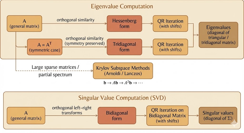 Figure: Overview of eigenvalue computation methods—from QR iteration to Krylov subspaces.
Background: Similarity and Triangular Matrices
Similar matrices: definition
Matrices \(A\) and \(B\) are similar if there exists an invertible matrix \(M\) such that \[ A \sim B \quad \Longleftrightarrow \quad A = M^{-1}BM. \] Similarity means “same linear map, different basis.”
Similar matrices have the same eigenvalues (two quick proofs)
Proof via characteristic polynomials \[ \det(A-\lambda I) = \det(M^{-1}BM-\lambda I) = \det\!\bigl(M^{-1}(B-\lambda I)M\bigr) = \det(M^{-1})\det(B-\lambda I)\det(M) = \det(B-\lambda I). \] So \(A\) and \(B\) have the same characteristic polynomial and thus the same eigenvalues.
Proof via eigenvectors mapping If \(Bx=\lambda x\), then \[ A(M^{-1}x)=M^{-1}BM(M^{-1}x)=M^{-1}Bx=\lambda(M^{-1}x), \] so \(A\) has the same eigenvalue \(\lambda\) with eigenvector \(M^{-1}x\).
Triangular matrices: eigenvalues are the diagonal entries
If \(T\) is upper triangular, then \(T-\lambda I\) is also upper triangular with diagonal entries \(t_{ii}-\lambda\). Therefore \[ \det(T-\lambda I)=\prod_{i=1}^n (t_{ii}-\lambda). \] So the eigenvalues of \(T\) are exactly \(t_{11},t_{22},\dots,t_{nn}\).
Key insight: If we can transform \(A\) into a triangular matrix \(T\) by similarity, we can read eigenvalues from the diagonal.
Shifting: \(A-sI\) keeps eigenvectors and shifts eigenvalues
If \(Ax=\lambda x\), then \[ (A-sI)x = Ax - sx = (\lambda-s)x. \] So \(A-sI\) has the same eigenvectors as \(A\), and its eigenvalues are \(\lambda-s\).
This “shift” idea is not cosmetic—it becomes the mechanism that accelerates iterative eigenvalue algorithms.
Motivation going forward
Our computational goal is now clear:
Use numerically stable similarity transformations to drive \(A\) toward (quasi-)triangular form, so the diagonal reveals the eigenvalues.
Computing Eigenvalues in Practice
QR iteration (core method)
The algorithm
Start with \(A_0=A\). For \(k=0,1,2,\dots\):
- Compute a QR factorization: \[ A_k = Q_k R_k, \] where \(Q_k\) is orthogonal (\(Q_k^\top Q_k=I\)) and \(R_k\) is upper triangular.
- Form the next iterate: \[ A_{k+1} = R_k Q_k. \]
Why QR iteration preserves eigenvalues (similarity proof)
From \(A_k=Q_kR_k\), we have \(R_k = Q_k^\top A_k\). Then \[ A_{k+1} = R_k Q_k = (Q_k^\top A_k)Q_k = Q_k^\top A_k Q_k. \] So \(A_{k+1}\) is orthogonally similar to \(A_k\), hence has the same eigenvalues. Repeating preserves eigenvalues at every step.
Why it converges toward triangular form
Intuitively, QR iteration repeatedly “pushes” mass upward because \(R_k\) is upper triangular. Over iterations, entries below the diagonal tend to shrink, and \(A_k\) approaches an upper triangular (or, in the real non-symmetric case, quasi-upper-triangular) form.
- For general real matrices, the stable endpoint is the real Schur form: upper quasi-triangular with \(1\times 1\) and \(2\times 2\) blocks on the diagonal (the \(2\times 2\) blocks represent complex-conjugate eigenpairs).
- For symmetric matrices, the Schur form is diagonal, and QR iteration can converge to an orthogonal diagonalization.
Shifted QR iteration (acceleration)
The shifted step
Pick a shift \(s_k\) and do:
- Factor: \[ A_k - s_k I = Q_k R_k, \]
- Update: \[ A_{k+1} = R_k Q_k + s_k I. \]
Why it still preserves eigenvalues
Compute: \[ A_{k+1} = R_k Q_k + s_k I = Q_k^\top(A_k - s_k I)Q_k + s_k I = Q_k^\top A_k Q_k. \] So shifted QR is still an orthogonal similarity transform; the shift changes convergence behavior, not the eigenvalues.
Wilkinson shift (practical choice)
A very effective choice is the Wilkinson shift, built from the trailing \(2\times 2\) block of \(A_k\). The idea is to choose \(s_k\) close to an eigenvalue “about to converge,” dramatically speeding deflation (making subdiagonal entries go to zero faster).
Preprocessing: Hessenberg and tridiagonal reduction
Why reduce first?
Running QR directly on a dense \(n\times n\) matrix costs too much per iteration. The fix is to first reduce \(A\) by orthogonal similarity into a nearly triangular structure that QR preserves:
- Upper Hessenberg form (general case): zeros below the first subdiagonal.
- Tridiagonal form (symmetric case): zeros except on the main diagonal and the first sub- and super-diagonals.
After reduction, each QR iteration is much cheaper, and the orthogonal transformations are numerically stable.
Symmetric case: tridiagonal is optimal
For symmetric \(A\), orthogonal reduction yields a symmetric tridiagonal matrix, which is the most compact “QR-friendly” form. The QR iterations then exploit that structure for both speed and stability.
Krylov subspace methods (large sparse matrices)
When \(A\) is huge and sparse, even Hessenberg QR can be too expensive. The alternative is to approximate eigenvalues using low-dimensional subspaces generated by repeated matrix-vector products.
Krylov subspace
Given a starting vector \(b\), \[ \mathcal{K}_k(A,b)=\text{span}\{b,\,Ab,\,A^2b,\,\dots,\,A^{k-1}b\}. \] This subspace tends to capture dominant spectral information (e.g., largest-magnitude eigenvalues) quickly.
Arnoldi vs. Lanczos
- Arnoldi (general \(A\)): builds an orthonormal basis of \(\mathcal{K}_k\) and produces a small \(k\times k\) upper Hessenberg matrix \(H_k\) that approximates \(A\) on the subspace.
- Lanczos (symmetric \(A\)): a specialization that yields a small tridiagonal matrix \(T_k\), cheaper and often more accurate per iteration.
Ritz values
The eigenvalues of the small projected matrix (\(H_k\) or \(T_k\)) are called Ritz values. They serve as approximations to eigenvalues of \(A\), often with excellent accuracy for extremal parts of the spectrum—without ever forming determinants or performing full matrix factorizations.
Computing Singular Values
SVD vs eigendecomposition: the connection
For any \(A\in\mathbb{R}^{m\times n}\), the singular value decomposition (SVD) is \[ A = U\Sigma V^\top, \] with \(U\) and \(V\) orthogonal and \(\Sigma\) diagonal (nonnegative entries \(\sigma_i\)).
The link to eigenvalues: \[ A^\top A = V\Sigma^2 V^\top, \] so the eigenvalues of \(A^\top A\) are \(\sigma_i^2\), and \(\sigma_i = \sqrt{\lambda_i(A^\top A)}\).
Practical note: forming \(A^\top A\) explicitly can square the condition number and amplify numerical issues, so high-quality SVD algorithms avoid relying on it directly.
Product of orthogonal matrices is orthogonal (proof)
If \(Q\) and \(U\) are orthogonal, then \[ (QU)^\top(QU) = U^\top Q^\top Q U = U^\top I U = I. \] So \(QU\) is orthogonal.
This matters because orthogonal transformations are the stable “currency” of numerical linear algebra: they preserve norms and avoid magnifying rounding errors.
Transformations preserve the SVD structure
Starting from \(A=U\Sigma V^\top\), if we apply orthogonal matrices \(Q_1, Q_2\), \[ Q_1 A Q_2 = Q_1(U\Sigma V^\top)Q_2 = (Q_1U)\Sigma (V^\top Q_2). \] Since \(Q_1U\) and \(Q_2^\top V\) remain orthogonal, we can transform \(A\) while preserving singular values—exactly the same philosophy as similarity transforms for eigenvalues.
Reduction strategies
To compute singular values efficiently, we reduce the problem to a structured form and then iterate:
- \(A \rightarrow\) bidiagonal form: Use Householder reflections on the left and right to reduce \(A\) to bidiagonal \(B\) (nonzeros only on diagonal and one adjacent diagonal). Then compute the SVD of \(B\) via specialized QR-like iterations (e.g., Golub–Kahan / implicit QR steps).
- \(A^\top A \rightarrow\) tridiagonal form: Since \(A^\top A\) is symmetric, it can be reduced to tridiagonal and then treated with symmetric eigenvalue methods; conceptually clean, but often avoided explicitly to reduce conditioning issues.
Same philosophy
Eigenvalues and singular values are computed by the same high-level recipe:
Reduce to a structured matrix using orthogonal transformations, then use iterative methods (QR-type or Krylov-type) to extract the spectrum.
Summary
- Determinants/characteristic polynomials define eigenvalues but are not practical numerical algorithms (instability + poor scaling).
- Closed-form eigenvalues stop being “general” at \(5\times 5\) because the characteristic polynomial is degree \(5+\) (Abel–Ruffini).
- Similarity transformations preserve eigenvalues; triangular matrices reveal eigenvalues on the diagonal.
- QR iteration is the workhorse: repeated orthogonal similarity drives a matrix toward (quasi-)triangular (Schur) form; shifts (e.g., Wilkinson) accelerate convergence.
- Pre-reducing to Hessenberg (general) or tridiagonal (symmetric) makes QR iterations efficient.
- For large sparse problems, Krylov methods (Arnoldi/Lanczos) approximate eigenvalues via Ritz values from a small projected matrix.
- Singular values follow the same philosophy: orthogonal reductions (bidiagonalization) plus iteration, closely connected to eigenvalues of \(A^\top A\) but computed more carefully in practice.