Theory-to-Repro: Linear Regression via Three Solvers

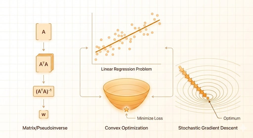
Linear regression is a single idea with multiple solution paths. In this note I solve the same least-squares objective three ways:

1. Pseudo-inverse (closed form)
2. Convex optimization (solver)
3. Stochastic gradient descent (iterative)

All three target \[ \min_w \; \|Xw - y\|_2^2. \]

Three ways to solve least squares

Problem setup

From the notebook, I used the Iris dataset and treated the class labels as numeric targets. Predictions are rounded to the nearest class. This is not a proper multi-class classifier, but it keeps the comparison focused on least squares.

from sklearn.datasets import load_iris
from sklearn.model_selection import train_test_split
import numpy as np

iris = load_iris()
X = iris['data']
y = iris['target']

# add bias column
X = np.hstack([np.ones((X.shape[0], 1)), X])
X_train, X_test, y_train, y_test = train_test_split(X, y, test_size=0.2)

Method 1: Pseudo-inverse (closed form)

The least-squares solution is \[ \hat{w} = X^+ y, \] where \(X^+\) is the Moore–Penrose pseudo-inverse (often computed via SVD). If \(X\) has full column rank, this matches \((X^T X)^{-1}X^T y\).

w = np.linalg.pinv(X_train) @ y_train
pred = X_test @ w

Pros: exact (up to floating point), fastest for small/medium problems.
Cons: can be expensive or unstable for huge or ill-conditioned matrices.

Method 2: Convex optimization (CVXPY)

We solve the same quadratic objective using a convex solver:

import cvxpy as cp

w = cp.Variable(X_train.shape[1])
objective = cp.Minimize(cp.sum_squares(X_train @ w - y_train))
problem = cp.Problem(objective)
problem.solve()

w = w.value
pred = X_test @ w

Pros: clean formulation, easy to add constraints or regularizers.
Cons: general solvers can be slower than the closed form.

Method 3: Stochastic gradient descent (SGD)

For mean-squared error, \[ \mathcal{L}(w)=\frac{1}{n}\sum_i (x_i^T w - y_i)^2, \] with gradient \[ \nabla_w \mathcal{L} = \frac{2}{n} X^T (Xw - y). \]

Mini-batch SGD updates \[ w \leftarrow w - \eta \, \nabla_w \mathcal{L} \] using small batches.

W = np.random.normal(0, 1, size=X_train.shape[1])
eta = 1e-2
batch = 2

for _ in range(epochs):
    for i in range(X_train.shape[0] // batch):
        xb = X_train[i*batch:(i+1)*batch]
        yb = y_train[i*batch:(i+1)*batch]
        y_pred = xb @ W
        grad = (2 / batch) * xb.T @ (y_pred - yb)
        W -= eta * grad

Pros: scales to large datasets, works online.
Cons: requires tuning (learning rate, batch size, epochs), converges approximately.

Comparison

Method	Objective	Exact?	Scales well?	Easy to constrain?
Pseudo-inverse	\(\|Xw-y\|_2^2\)	Yes	Medium	No
Convex solver	\(\|Xw-y\|_2^2\)	Yes (to tol)	Medium	Yes
SGD	\(\|Xw-y\|_2^2\)	Approx	Yes	Yes (via regularization)

Takeaways

• All three methods solve the same least-squares problem.
• Pseudo-inverse is the cleanest theoretical solution.
• Convex optimization is the easiest way to add constraints.
• SGD is the most scalable for large data.

Next step: replace rounded regression with proper multi-class logistic regression and compare accuracy + calibration.