Goodfellow Deep Learning — Chapter 13: Linear Factor Models
Source: Deep Learning Book - Chapter 13: Linear Factor Models
Latent Factors
The latent factors serve as explanatory variables for the observed data and are not directly observable.
\[ h \sim p(h) \]
\(p(h)\) is the factor distribution, satisfies \(p(h)=\prod_ip(h_i)\).
Next, given the latent factors, we sample the real-valued observed variables.
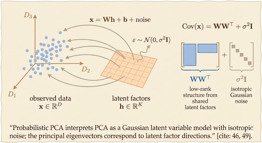
\[ x=Wh+b+\text{noise} \]
PCA and Factor Analysis
In factor analysis, the prior probability is a Gaussian distribution with variance as I (identity matrix).
\[ h \sim \mathcal{N}(h;0,I) \]
The use of latent factor is to detect the dependencies of each component of x (\(x_i\)).
We can see x follows multivariable normal distribution:
\[ x\sim \mathcal{N}(x;b,WW^\top+\psi) \]
- \(\mathbb{E}[h]=0\)
- \(\mathbb{E}[\text{noise}]=0\)
- \(\mathbb{E}[x]=\mathbb{E}[Wx+b+\text{noise}]=b\)
- The covariance takes the form \(WW^\top+\Psi\) because correlations among observed variables are explained by shared latent factors, while the remaining variability is attributed to independent noise.
To use PCA, we set \(\psi\) to a constant \(\sigma^2\):
\[ x\sim\mathcal{N}(x;b,WW^\top+\sigma^2 I) \]
Equally,
\[ X =Wh+b+\sigma z\\ z\sim \mathcal{N}(0,I) \]
This model provides a probabilistic interpretation of PCA. When the noise covariance is isotropic, i.e., maximum likelihood estimation of the Gaussian latent variable model yields a solution in which the columns of W span the same subspace as the principal eigenvectors of the data covariance matrix.
Thus, probabilistic PCA recovers the same principal directions as classical PCA, which is based on eigenvalue decomposition.
ICA
Independent Component Analysis (ICA) is a linear factor model whose goal is to recover statistically independent latent sources from observed data.
It assumes that the observed vector x is generated by a linear mixing of latent variables h, typically written as \(x = Wh\) (sometimes with noise), and the key modeling assumption is that the components of h are independent and non-Gaussian.
Unlike probabilistic PCA and factor analysis, ICA does not usually specify an explicit probability distribution p(x). Instead, it focuses on finding a transformation that makes the recovered components as independent as possible, often by maximizing non-Gaussianity or minimizing statistical dependence. Because of this, many ICA variants are not generative models in the strict probabilistic sense.
ICA is particularly well suited for source separation problems, such as separating mixed audio signals or neural signals, where the latent variables correspond to real underlying sources. The requirement that p(h) be non-Gaussian is essential for identifiability; if the latent variables were Gaussian, the model would reduce to PCA and the independent components would not be uniquely determined.
A classic example is the cocktail party problem, where multiple people speak simultaneously and several microphones record mixtures of their voices. Each microphone captures a linear combination of the original speech signals. ICA assumes that the underlying source signals are statistically independent and non-Gaussian, and aims to recover these original sources from the observed mixtures. In this setting, the latent variables correspond to real physical sources, such as individual speakers.
Another example discussed is the analysis of neural signals, such as EEG recordings. Electrodes placed on the scalp measure mixtures of signals originating from different brain regions, as well as strong artifacts from sources like eye movements and heartbeats. ICA can be used to separate these mixed signals into independent components, allowing researchers to isolate brain activity from physiological noise. Here again, the latent variables represent meaningful, independent signal sources.
The book emphasizes that many ICA methods do not explicitly model the data distribution p(x). Instead, they focus on finding a transformation between x and h that makes the components of h as independent as possible. Because of this, ICA is often used as a signal separation and analysis tool, rather than as a fully probabilistic generative model.
Finally, the book highlights that non-Gaussianity of the latent variables is essential for ICA to be identifiable. If the latent variables were Gaussian, the model would reduce to PCA, and the independent components would not be uniquely determined.
SFA
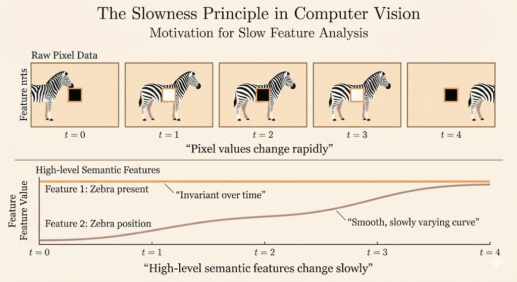
Slow Feature Analysis is from the Slowness Principle.
The slowness principle states that meaningful underlying factors of variation in the data tend to change slowly over time.
Slow Feature Analysis learns feature functions whose outputs vary as slowly as possible across time, subject to suitable constraints.
For example, in a computer vision setting, individual pixel values may change rapidly over time. If a zebra moves from left to right across an image, pixels at fixed locations may quickly switch from white to black and back again. However, higher-level semantic properties, such as whether the image contains a zebra, remain invariant, while other properties, such as the position of the zebra, tend to change much more slowly.
Regularization
We introduce a regularization term to bias the model toward learning slowly varying features over time.
We add the following penalty item to the loss function:
\[ \lambda \sum_tL(f^{t+1},f^t) \]
- \(\lambda\): hyper-parameter of the strength of the slowness regularization
- f: the slow feature extraction
- t: the index of the time sequence
SFA is one of the most practical ways to put the slowness principle into action. Instead of using complex models, SFA relies on a simple linear feature extractor that can be trained with a closed-form solution, making it both fast and efficient.
Like some variants of ICA, SFA is not a generative model. It does not try to explain how the data was generated. Rather, it focuses on learning a linear mapping from the input space to a feature space, without assuming any prior over the features or imposing a probability distribution p(x) on the inputs.
SFA Algorithm
Optimization problem: learned features should vary as little as possible between consecutive time steps. In other words, the model is encouraged to extract signals that evolve slowly across time rather than rapidly fluctuating measurements.
\[ \min_{\theta}\t\mathbb{E}_t(f(x^{t+1})_i-f(x^t)_i)^2 \]
Constraints:
- \(\mathbb{E_t}f(x^t)_i=0\) enforces a zero-mean constraint on each feature. This prevents the model from learning trivial constant outputs, which would be perfectly slow but carry no useful information.
- \(\mathbb{E}_t[f(x^t)_i^2]=1\) fixes the variance of each feature to one. This avoids degenerate solutions where features collapse toward zero, again producing artificially slow but uninformative representations.
Today, Slow Feature Analysis is rarely used as a standalone algorithm in practice. However, its central idea—that meaningful representations should vary slowly over time—has become a foundational principle in modern self-supervised learning. While deep neural networks have largely replaced SFA’s linear, closed-form formulation, the slowness principle now appears implicitly in video-based representation learning, contrastive learning, and world models, where temporal coherence and invariance serve as key inductive biases. In this sense, SFA’s influence has grown even as its original form has faded.
Sparse Coding
Like other linear factor models, sparse coding represents the input x as a linear combination of latent factors, plus noise.
\[ p(x|h)=\mathcal{N}(x,Wh+b,\frac{1}{\beta}I) \]
The distribution \(p(h)\) is typically chosen to be sharply peaked around zero, which encourages most latent variables to be inactive and leads to sparse representation.
For example, a Laplace prior with sparse penalty parameter \(\lambda\):
\[ p(h_i)=\mathcal{Laplace}(h_i;0,\frac{2}{\lambda}) \]
It is not feasible to train sparse coding models using maximum likelihood. Instead, training proceeds by alternating between inferring the sparse latent variables and updating the dictionary parameters.
\[ h^*=f(x)=\arg\max_h p(h|x)=\\ \arg\max_h p(h|x)=\\ \arg\min_h \lambda ||h_i||_1+\beta||x-Wh||_2^2 \]
Adding an L1 norm penalty on h encourages most latent variables to be zero, resulting in sparse representations.
A Flow Interpretation of PCA
The encoder can be represented as:
\[ h=f(x)=W^\top(x-\mu) \]
Then the decoder can regenerate \(\hat{x}\):
\[ \hat{x}=g(h)=Vh+b \]
The linear encoder and decoder that can minimize \(\mathbb{E}[||x-\hat{x}||_2^2]\) is:
- \(V=W\)
- \(\mu=b=\mathbb{E}[x]\)
- The columns of W are the orthogonal basis, and the space they span are the same space as \(C=\mathbb{E}[(x-\mu)(x-\mu)^\top]\)
If \(x\in \mathbb{R}^D\), \(h\in \mathbb{R}^d\), and \(d< D\), the optimal reconstruction error is:
\[ \min \mathbb{E}[||x-\hat{x}||_2^2]=\sum_{i=d+1}^D\lambda_i \]
So if the rank of the covariance matrix is d, then \(\lambda_{d+1}, \dots, \lambda_D\) are all 0, so the reconstruction error is 0.