Goodfellow Deep Learning — Chapter 14: Autoencoders
Source: Deep Learning Book - Chapter 14: Autoencoders
What is an Autoencoder?
An autoencoder is a neural network trained to copy its input to its output through a bottleneck representation. This seemingly trivial task forces the network to learn useful features.
The architecture consists of two components:
- Encoder: \(h = f(x)\) compresses input x into a lower-dimensional code h
- Decoder: \(r = g(h)\) reconstructs the input from the code
The bottleneck layer h forces the network to learn a compressed representation that captures the essential structure of the data.
Undercomplete Autoencoders
An undercomplete autoencoder learns useful features by constraining the code dimension to be smaller than the input:
\[ \dim(h) < \dim(x) \]
Training objective: Minimize reconstruction error
\[ L(x, g(f(x))) \]
where L is a loss function measuring the difference between the original input x and the reconstruction \(g(f(x))\). Common choices include mean squared error.
Connection to PCA:
When both encoder and decoder are linear and L is squared error, the undercomplete autoencoder learns the same subspace as Principal Component Analysis (PCA). The autoencoder generalizes PCA to nonlinear transformations.
Regularized Autoencoders
To prevent the autoencoder from simply learning the identity function, various regularization strategies encourage learning meaningful representations.
Sparse Autoencoders
Sparse autoencoders add a sparsity penalty \(\Omega(h)\) to encourage most activations in h to be zero:
\[ L(x, g(f(x))) + \Omega(h) \]
Purpose: Sparsity prevents trivial identity mappings and encourages the network to discover meaningful structure. Sparse representations are particularly useful for downstream tasks like classification.
Why Sparse Autoencoders Differ from Weight Decay
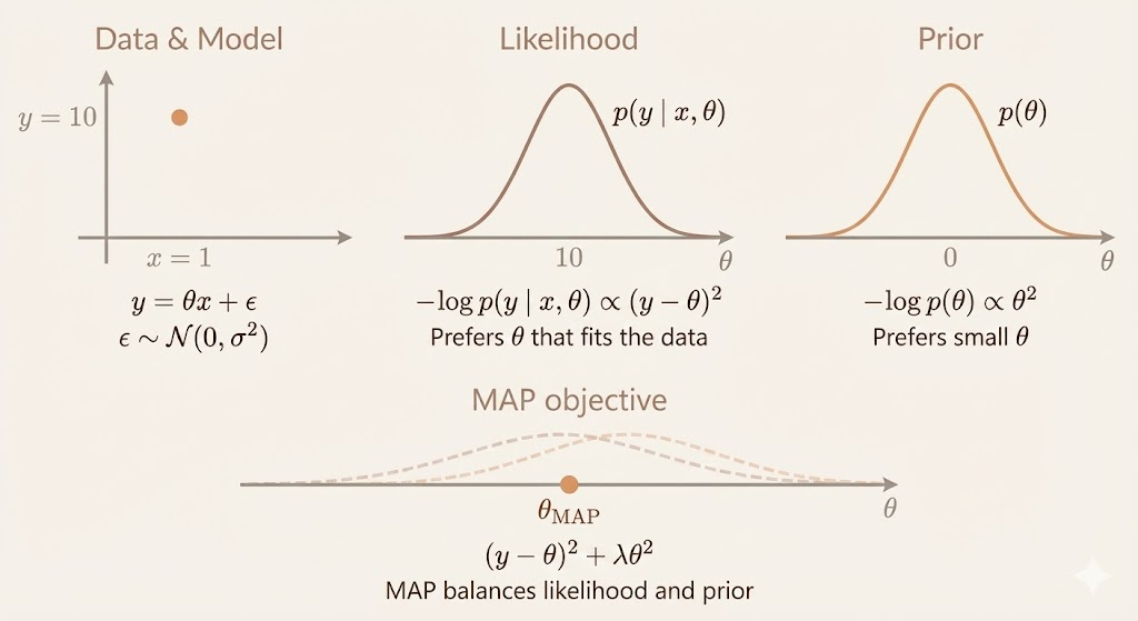
Standard regularization (like weight decay) can be interpreted in a Bayesian framework as Maximum A Posteriori (MAP) estimation:
\[ \max_\theta \log p(x \mid \theta) + \log p(\theta) \]
where: - \(\log p(x \mid \theta)\) is the data likelihood - \(\log p(\theta)\) is a prior over parameters
Key difference: Sparse autoencoders don’t admit this interpretation because the sparsity penalty depends on the data through \(h = f(x)\). By definition, a prior cannot depend on observed data, so the sparsity penalty is not a true Bayesian prior over parameters.
Probabilistic Interpretation via Latent Variables
Though not equivalent to a Bayesian prior, we can build intuition by comparing to latent-variable models. Consider:
\[ \log p_{\text{model}}(x) = \log \sum_h p_{\text{model}}(h, x) \]
Using a point estimate for h:
\[ \log p_{\text{model}}(h, x) = \log p_{\text{model}}(h) + \log p_{\text{model}}(x \mid h) \]
From this perspective: - Reconstruction loss \(\leftrightarrow\) conditional likelihood \(\log p(x \mid h)\) - Sparsity penalty \(\leftrightarrow\) preference over latent codes h
Sparsity as Laplace Distribution
To encourage sparsity, assume each latent variable follows a Laplace distribution:
\[ p_{\text{model}}(h_i) = \frac{\lambda}{2} e^{-\lambda |h_i|} \]
Taking the negative log-likelihood:
\[ \log p_{\text{model}}(h) = \sum_i \left( \lambda |h_i| - \log \frac{\lambda}{2} \right) = \Omega(h) + \text{const} \]
Thus, an L1 sparsity penalty naturally arises as the negative log-probability of a Laplace-distributed latent variable. This shows that sparsity corresponds to a meaningful statistical assumption, not an arbitrary constraint.
Important caveat: Although this resembles a log-prior, it’s not a true Bayesian prior because it depends on the data through \(h(x)\).
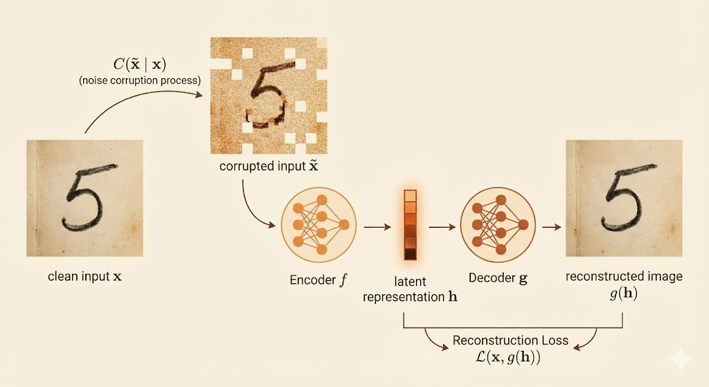
Denoising Autoencoders (DAE)
Denoising autoencoders learn to remove corruption rather than simply copying the input.
Training procedure:
- Sample a clean input x from the data
- Sample a corrupted version \(\tilde{x}\) from corruption distribution \(C(\tilde{x} \mid x)\)
- Train to minimize \(L(x, g(f(\tilde{x})))\)
Corruption process: Typically Gaussian noise
\[ C(\tilde{x}|x) = \mathcal{N}(\mu=x, \Sigma=\sigma^2 I) \]
Learning objective: Estimate the reconstruction distribution
\[ p_{\text{reconstruct}}(x|\tilde{x}) = p_{\text{decoder}}(x|h) \]
where h is given by the encoder \(f(\tilde{x})\) applied to the corrupted input.
Geometric interpretation:
The denoising autoencoder learns the local structure of the data distribution rather than explicitly modeling the density. When corruption noise is small and Gaussian, the optimal reconstruction function has a precise probabilistic meaning:
The residual vector \(g(f(x)) - x\) estimates a vector field proportional to the score of the data distribution:
\[ g(f(x)) - x \propto \nabla_x \log p_{\text{data}}(x) \]
This means the autoencoder learns to point toward regions of higher density, implicitly capturing the manifold structure.
Penalizing Derivatives (Contractive Penalty)
Another regularization strategy penalizes the sensitivity of the representation to input perturbations:
\[ \Omega(h,x) = \lambda \sum_i \|\nabla_x h_i\|^2 \]
This forces the encoder to learn representations that are insensitive to small changes in the input—a property useful for robustness and generalization.
Architecture: Depth and Width
While a single-layer encoder may be expressive enough (universal approximation theorem), deep autoencoders offer significant advantages:
- More compact representations: Hierarchical feature learning
- Structured encodings: Compositions of simpler features
- Better optimization: When combined with regularization (sparsity, contractive penalties)
Depth allows the network to learn abstract, compositional representations that are more efficient than shallow alternatives.
Manifold Learning Perspective
Autoencoders can be understood as learning the geometric structure of the data distribution, based on the assumption that high-dimensional data lie near a low-dimensional manifold embedded in the input space.
Two Competing Forces
Autoencoder training is driven by two complementary objectives:
- Reconstruction objective: Accurately reconstruct training examples, anchoring the learned function near the data manifold
- Regularization: Encourage invariance to perturbations that move inputs off the manifold (via denoising, sparsity, or contractive penalties)
Together, these forces lead the encoder to become: - Sensitive to directions tangent to the data manifold - Insensitive to directions orthogonal to the manifold
Local Manifold Approximation
Locally, the data manifold can be approximated by a tangent plane. The learned representation effectively provides a coordinate system aligned with these locally valid directions of variation.
Denoising vs Contractive:
- Denoising autoencoders: Learn to map corrupted inputs back toward high-density regions, implicitly capturing manifold geometry
- Contractive autoencoders: Explicitly penalize the Jacobian to encourage robustness to perturbations
Unlike non-parametric manifold learning methods, autoencoders learn a parametric mapping that generalizes beyond training samples, enabling modeling of complex, highly curved manifolds.
Contractive Autoencoders (CAE)
A contractive autoencoder penalizes the Frobenius norm of the Jacobian to encourage local contraction:
\[ \Omega(h) = \lambda \left\|\frac{\partial f(x)}{\partial x}\right\|_F^2 \]
Interpretation:
- If the Jacobian norm is small, nearby inputs are mapped to nearby representations
- The encoder behaves like a local contraction mapping with Lipschitz constant < 1
- This prevents the mapping from amplifying input perturbations
Two Competing Forces in CAE
- Reconstruction loss: Encourages sensitivity to directions where data varies
- Contraction penalty: Encourages insensitivity to irrelevant directions
This balance prevents trivial constant solutions while enforcing meaningful invariances.
Relation to Manifold Learning
CAE can be interpreted as a manifold learning method:
- Data lie near a low-dimensional manifold
- The Jacobian’s dominant singular vectors correspond to tangent directions of the manifold
- Directions with small singular values correspond to noise or off-manifold variations
Thus, CAE learns a local linear approximation of the manifold at each data point.
Predictive Sparse Decomposition (PSD)
Traditional sparse coding requires expensive optimization at test time. Predictive Sparse Decomposition introduces a parametric predictor \(f(x)\) that approximates the optimal sparse code.
Training objective:
\[ \text{minimize} \quad \|x - g(h)\|^2 + \lambda \|h\|_1 + \gamma \|h - f(x)\|^2 \]
where: - \(\|x - g(h)\|^2\): Reconstruction loss - \(\lambda \|h\|_1\): Sparsity penalty - \(\gamma \|h - f(x)\|^2\): Prediction consistency
Key innovation: PSD separates representation definition from inference computation:
- The representation h is still defined by the sparse coding objective
- But inference is amortized into a fast feedforward computation through \(f(x)\)
At test time, a single forward pass through \(f(x)\) produces an approximate sparse representation, eliminating the need for expensive optimization.
Applications: Dimensionality Reduction and Semantic Hashing
Autoencoders are commonly applied to:
- Dimensionality reduction: Learning compact representations that preserve semantic similarity
- Information retrieval: When codes are low-dimensional or binary, they enable efficient similarity search
Semantic hashing: Binary autoencoder codes allow fast retrieval with: - Reduced memory usage - Fast query time via Hamming distance - Preserved semantic similarity
These representations improve generalization and make large-scale retrieval practical in domains like images, text, and audio.
Why it works: The learned codes capture high-level semantic structure while discarding irrelevant variations, enabling meaningful similarity comparisons in the compressed space.