MIT 18.065 Lecture 10: Survey of Difficulties of Ax=b
Ax=b Difficulties
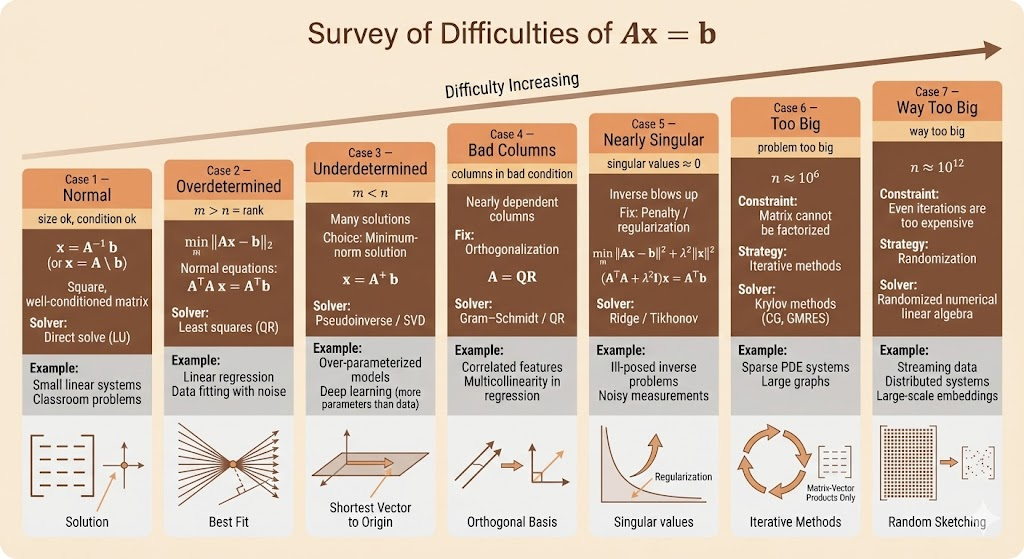
- \(x=A^+b\)
- size ok, condition( \(\frac{\sigma_1}{\sigma_r}\) ) ok, \(x=A\backslash b\)
- \(m\gt n =r\),
- A is overdetermined, there is no solution for x
- use least square to find \(\hat{x}\)
- \(A^\top A \hat{x}=A^\top b\)
- \(m\lt n\)
- A is underdetermined, x has many solutions
- we pick the one with min norm
- \(x=A^+b\)
- columns in bad conditions
- Gram-schmidt , factorize A to orthogonal
- A=QR
- Nearly singular
- singular values very close to 0
- the reverse will be quite big
- add penalty to the solution
- \(\min ||Ax-b||^2+\delta^2||x||^2\)
- Problem too big
- e.g. \(10^6\),iteratively
- Krylov
- way too big
- e.g. \(10^{12}\)
- randomize linear algebra
- use probability to sample the matrix, work with samples
In deep learning, we are typically in an underdetermined regime (m < n), where infinitely many solutions exist. The key question is not whether a solution exists, but which solution the optimization algorithm selects. In practice, optimization methods such as (stochastic) gradient descent exhibit an implicit bias toward low-norm or simple solutions, even without explicit regularization.
Ill-Conditioned Problem
The solution is to solve \(\min ||Ax-b||_2^2+\delta^2||x||_2^2\).
Let \(A^*=\begin{bmatrix}A\\\delta I\end{bmatrix},b^*=\begin{bmatrix}b\\0\end{bmatrix},A^*x=b^*\).
so the least square solution of \(A^*x=b^*\) turns out to be \(\min||Ax-b||^2+\delta^2||x||^2\).
The normal equation is \((A^*)^\top A^* x=(A^*)^\top b^* \Rightarrow (A^\top A+\delta^2 I)x=A^\top b\).
\(x=(A^\top A+\delta^2I)^{-1}A^\top b\)
When \(\lim_{\delta \to 0}\), it turns out to be pseudo inverse solution.
Role of the Moore–Penrose Pseudo-Inverse in Different Regimes
| Regime | System Properties | Existence of Solution | What A^+ b Represents | Key Interpretation |
|---|---|---|---|---|
| Square, full rank | m = n, A invertible | Unique exact solution | \(A^{-1} b\) | Pseudo-inverse reduces to the true inverse |
| Overdetermined | \(m > n, \mathrm{rank}(A)=n\) | No exact solution | Least-squares solution | Minimizes ||Ax - b||_2 |
| Underdetermined | \(m < n, \mathrm{rank}(A)=m\) | Infinitely many solutions | Minimum-norm solution | Selects the smallest-\(\ell_2\) solution among all feasible ones |
| Rank-deficient | \(\mathrm{rank}(A) < \min(m,n)\) | Non-unique or unstable | Stable, minimum-norm solution | Removes null-space ambiguity |
| Ill-conditioned | Small singular values | Sensitive to noise | Truncated / damped inverse | Filters directions with little information |
| Penalty → 0 | \(\text{Ridge with}\quad \lambda \to 0\) | Well-defined limit | \(A^+ b\) | Pseudo-inverse is the zero-regularization limit |
| Gradient descent (init = 0) | Linear least squares | Implicitly chosen | \(A^+ b\) | Optimization bias toward minimum-norm |