Chapter 4.3: Linear Optimization
Convex Optimization Textbook - Chapter 4.3 (page 165)
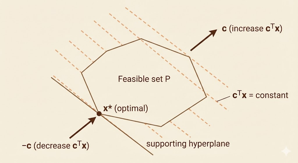
The General Form
\[ \begin{aligned} \text{minimize}&\quad c^\top x+d \\ \text{subject to}&\quad Gx \preceq h \\&\quad Ax=b \end{aligned} \]
The constraints define a polyhedron feasible set, the level curves of \(c^\top x\) are hyperplanes orthogonal to c.
The optimal point \(x^*\) is the point in feasible set as far as possible in the direction of -c.
Convert constraints to standard form:
Say we have constraints: - \(Ax\succeq b\)
we can convert it to \(-Ax\preceq -b; G=-A;Gx \preceq -b\)
The standard form
\[ \begin{aligned} \text{minimize} &\quad c^\top x \\ \text{subject to}&\quad Ax=b\\ &\quad x \succeq0 \end{aligned} \]
Example
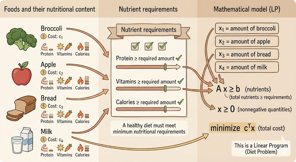
Diet Problem
The Diet Problem asks how to choose a combination of foods that meets all nutritional requirements at minimum total cost.
Each available food provides certain amounts of nutrients (such as protein, vitamins, or calories) per unit and has an associated cost. A healthy diet must supply at least a required minimum amount of each nutrient, while food quantities must be nonnegative.
The goal is to determine how much of each food to consume so that all nutritional constraints are satisfied and the total cost is minimized.
Decision variables
- \(x_i \ge 0:\) quantity of food i to include in the diet
Data
- \(a_{ij}:\) amount of nutrient j provided by one unit of food i
- \(b_j\): minimum required amount of nutrient j
- \(c_i\): cost per unit of food i
\[ \begin{aligned} \text{minimize} \quad & c^\top x \\ \text{subject to} \quad & A x \succeq b \\ & x \succeq 0 \end{aligned} \]
Piecewise minimization
\[ \text{minimize}\quad \max_{i=1,\dots,m}(a_i^\top x+b_i) \]
equivalent LP:
\[ \begin{aligned} \text{minimize}&\quad t\\ \text{subject to}&\quad a_i^\top x+b_i\le t,i=1,\dots,m \end{aligned} \]
Chebyshev center of a polyhedron
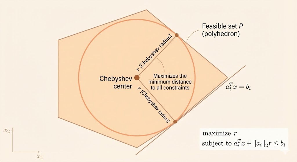
Feasible set
\[ \mathcal{P}=\{x|a_i^\top x \le b_i, \quad i=1,\dots,m\} \]
Largest ball inside feasible set
\[ \mathcal{B}=\{x_c+u| \, ||u||\le r\} \]
\[ \sup\{a_i^\top (x_c+u) \,|\, ||u||_2\le r\}=a_i^\top x_c+r||a_i||_2\le b_i \]
LP Form
\[ \begin{aligned} \text{maximize} &\quad r\\ \text{subject to} &\quad a_i^\top x+r||a_i||_2\le b_i\, i=1,\dots,m \end{aligned} \]
Dynamic Activity Planning
Linear Fractional Program
\[ \begin{aligned} \text{minimize}&\quad f_0(x)\\ \text{subject to}&\quad Gx \preceq h\\ &\quad Ax=b \end{aligned} \]
Linear Fractional
\[ f_0(x)=\frac{c^\top x+d}{e^\top x+f}\quad \text{dom }f_0(x)=\{x|e^\top x+f \gt 0\} \]
equivalent to LP by introducing variables \(y,z\)
- \(z=\frac{1}{e^\top x+f}\)
- \(y=xz\)
\[ \begin{aligned} \text{minimize}&\quad c^\top y+dz\\ \text{subject to}&\quad Gy\preceq hz\\ &\quad Ay=bz\\ &\quad e^\top y+fz=1\\ &\quad z\gt0 \end{aligned} \]
Linear fractional optimization problems can be converted to linear programs by normalizing variables with respect to the denominator.
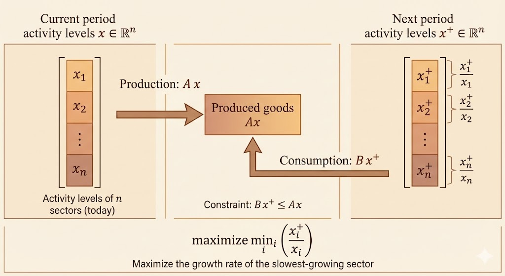
Example Von Neumann model of growing economy
\[ \begin{aligned} \text{maximize}&\quad \min_{i=1,\dots,n}x_i^+/x_i\\ \text{subject to}&\quad x\succeq 0,x^+\succeq 0,Bx^+\preceq Ax \end{aligned} \]
- Models a multi-sector economy over two consecutive periods: the current period and the next period.
- Decision variables:
- \(x \in \mathbb{R}^n\): activity levels in the current period
- \(x^+ \in \mathbb{R}^n\): activity levels in the next period
- Production and consumption:
- \(Ax:\) goods produced by current-period activities
- \(Bx^+:\) goods required to support next-period activities
- Feasibility constraint: \(Bx^+ \le Ax\) Goods produced in the current period must be sufficient to support activities in the next period.
- Nonnegativity constraints: \(x \ge 0, \quad x^+ \ge 0\)
- Growth rates:
- Each sector i has a growth rate \(x_i^+ / x_i\).
- Objective: \(\max \; \min_i \left( \frac{x_i^+}{x_i} \right)\) Maximize the growth rate of the slowest-growing sector.
- Interpretation:
- Ensures balanced growth across all sectors.
- Prevents any sector from becoming a bottleneck.
- Optimization structure:
- The objective is a max–min of linear fractional functions.
- The problem is quasiconvex and can be solved via bisection, where each feasibility check reduces to a linear program.