Goodfellow Deep Learning — Chapter 12.4: NLP Applications
N-gram Models
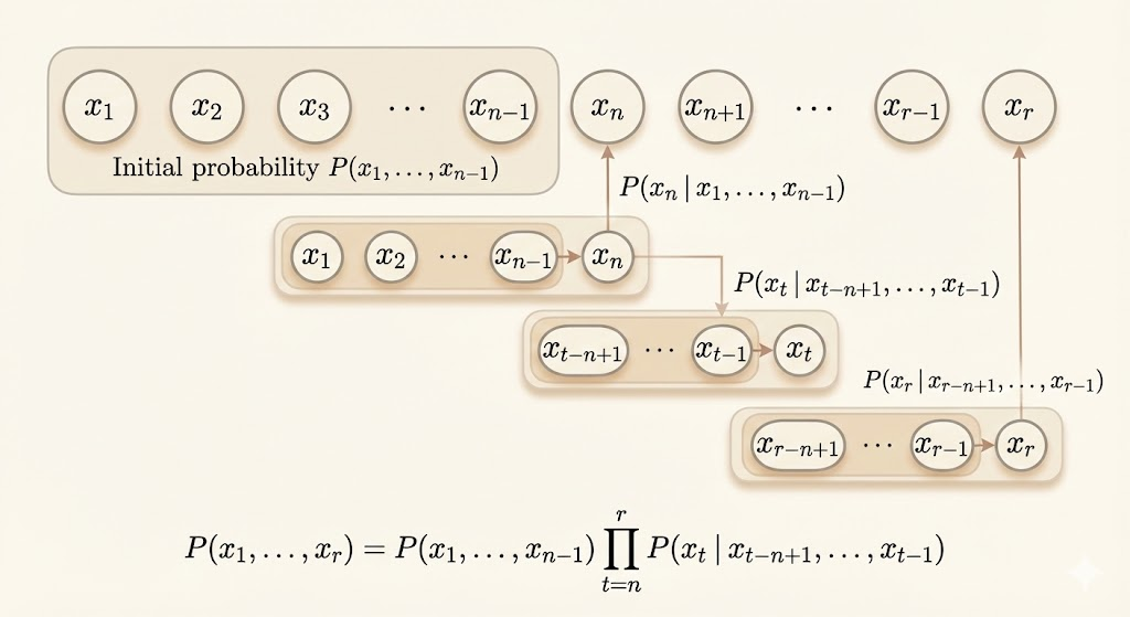
N-gram models were the earliest successful language models, and they are fixed-length labeling models.
N-gram defines a conditional probability of the current token given the previous \(n-1\) tokens:
\[ P(x_1,\dots,x_\tau)=P(x_1,\dots,x_{n-1})\prod_{t=n}^\tau P(x_t|x_{t-n+1},\dots,x_{t-1}) \]
Common n-gram orders: - \(n=1\) (unigram) - \(n=2\) (bigram) - \(n=3\) (trigram)
In practice, both n-gram and \((n-1)\)-gram models are estimated, since the conditional probability requires both joint distributions:
\[ P(x_t|x_{t-n+1},\dots,x_{t-1})=\frac{P_n(x_{t-n+1},\dots,x_t)}{P_{n-1}(x_{t-n+1},\dots,x_{t-1})} \]
This is just \(P(A|B)=P(A,B)/P(B)\).
For example, in a trigram model (\(n = 3\)), to compute the conditional probability \(P(\text{run} \mid \text{The dog})\), we use:
\[ P(\text{run} \mid \text{The dog}) = \frac{P(\text{The dog run})}{P(\text{The dog})} \]
Therefore, estimating trigram probabilities requires estimating bigram (\((n-1)\)-gram) probabilities as well.
Sparsity
A key limitation of n-gram models is data sparsity: if an \((n-1)\)-gram context is unseen (in training set), the conditional probability is undefined; if the context is seen but the corresponding n-gram has zero count, the conditional probability is zero and the log-likelihood becomes \(-\infty\).
Smoothing techniques address data sparsity in n-gram language models by redistributing probability mass from observed n-grams to unseen but plausible ones, preventing undefined probabilities and negative-infinite log-likelihoods.
Curse of Dimensionality
N-gram language models suffer from the curse of dimensionality, since the number of possible contexts grows exponentially with the n-gram order.
Suppose we have 50,000 words and \(n=5\), in theory there are \(50000^5 = 3.125 \times 10^{23}\) possibilities.
Neural Language Models (NLM)
Neural language models (NLM) mitigate the curse of dimensionality by mapping discrete words to continuous, low-dimensional representations.
Unlike n-gram models, neural language models learn distributed representations that capture similarities between tokens. As a result, semantically related words such as “cat” and “dog” are mapped to nearby representations, allowing training examples involving one word to improve predictions involving the other.
Word Embeddings
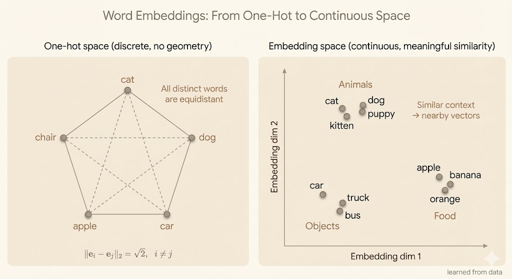
We call the word representations word embeddings. Word embeddings map words into a low-dimensional continuous feature space.
In the original one-hot representation, each word is represented by a one-hot vector, and the Euclidean distance between any two distinct words is \(\sqrt{2}\).
In contrast, in the embedding space, words that occur in similar contexts are located close to each other.
High-Dimensional Output
In most NLP applications, models generate tokens rather than characters. With a large vocabulary, the output layer must represent a probability distribution over many possible tokens, making the computation and parameterization expensive.
Assume \(h\) is the top hidden layer, then we use \(W\) and \(b\) to transform \(h\) to \(\hat{y}\):
\[ \begin{align} a_i &= b_i+\sum_jW_{i,j}h_j \quad \forall i\in \{1,\dots,|\mathbb{V}|\}\\ \hat{y}_i &= \frac{e^{a_i}}{\sum_{i}^{|\mathbb{V}|}e^{a_i}} \end{align} \]
If the hidden layer \(h\) has \(h_n\) units, computing the output logits requires \(O(|\mathbb{V}| \cdot h_n)\) operations.
In practice, the vocabulary size \(|\mathbb{V}|\) is often on the order of hundreds of thousands, while \(h_n\) can be in the thousands. As a result, computing the full softmax over the vocabulary becomes computationally expensive.
Using Short Lists
In neural language models, generating words typically requires computing a softmax over the entire vocabulary. When the vocabulary size \(|\mathbb{V}|\) is very large (often tens or hundreds of thousands of words), the output layer becomes computationally expensive, since both the number of parameters and the cost of computing logits and normalization scale as \(O(|\mathbb{V}| \cdot h_n)\), where \(h_n\) is the dimensionality of the top hidden layer.
To reduce this cost, the short-list method partitions the vocabulary into two disjoint subsets:
- A short list (\(L\)) consisting of the most frequent words
- A tail list (\(T = \mathbb{V} \setminus L\)) containing the remaining rare words
For words in the short list, the neural language model computes an exact softmax over \(L\), allowing accurate modeling of frequent words that account for most of the probability mass in natural language. For words in the tail list, probabilities are not computed using a full neural softmax; instead, they are approximated using simpler models, typically n-gram language models.
The model therefore learns to predict: - The probability that the next word belongs to the short list, and - The conditional probability of each word within the short list or the tail list, depending on which subset it belongs to.
This approach significantly reduces computational cost while maintaining good performance, since frequent words dominate language usage and benefit most from expressive neural modeling, whereas rare words contribute relatively little to the overall probability mass.
However, the short-list method is fundamentally an engineering approximation rather than a principled solution. It still relies on a discrete vocabulary and does not eliminate the need for large output layers entirely. As a result, it serves as an intermediate step toward more scalable approaches such as hierarchical softmax, sampled softmax, and noise-contrastive estimation.
Hierarchical Softmax
In neural language models with large vocabularies, computing a full softmax over all words is computationally expensive, since the cost scales linearly with the vocabulary size \(|\mathbb{V}|\). Hierarchical softmax addresses this problem by factorizing the softmax computation using a tree-based structure.
In hierarchical softmax, the vocabulary is organized as a binary (or multi-branch) tree. Each leaf node corresponds to a word in the vocabulary, while each internal node represents a binary decision. Predicting a word is equivalent to traversing a unique path from the root of the tree to the corresponding leaf node.
Instead of computing probabilities for all words, the model computes a sequence of conditional probabilities along this path. Each internal node performs a binary classification, typically using a sigmoid function. The probability of a word is therefore expressed as the product of these binary decisions along its path.
Because the depth of a balanced tree is approximately \(\log |\mathbb{V}|\), hierarchical softmax reduces the computational complexity of predicting a word from \(O(|\mathbb{V}| \cdot h_n)\) to \(O(\log |\mathbb{V}| \cdot h_n)\), where \(h_n\) is the dimensionality of the top hidden layer. This reduction applies during both training and inference.
The effectiveness of hierarchical softmax depends strongly on the structure of the tree. In theory, information-theoretic constructions such as Huffman coding can minimize the expected computation by assigning shorter paths to frequent words. In practice, however, the tree structure is usually predefined and not learned jointly with the language model parameters.
While hierarchical softmax provides a principled and substantial computational improvement over the standard softmax, its performance can be sensitive to poor tree design. As a result, although it improves efficiency, hierarchical softmax is often outperformed in practice by sampling-based methods such as sampled softmax or noise-contrastive estimation.
Importance Sampling
This section analyzes the computational bottleneck of the softmax output layer in neural language models by explicitly deriving the gradient of the log-likelihood. The derivation shows that the gradient decomposes into a positive term that increases the score of the target word and a negative term that requires taking an expectation over the entire vocabulary. The latter dominates the computational cost, scaling linearly with the vocabulary size.
To reduce this cost, Monte Carlo methods are considered to approximate the negative phase using sampling. Since sampling directly from the model distribution is expensive, importance sampling is introduced, where samples are drawn from a simpler proposal distribution and reweighted to correct for the mismatch. This yields an unbiased estimator of the gradient in theory.
However, the section emphasizes that importance sampling is often ineffective in practice for neural language models. Computing accurate importance weights still depends on the model probabilities, which themselves require evaluating the softmax. Moreover, poorly chosen proposal distributions lead to high-variance estimates, making training unstable. These difficulties are exacerbated in language modeling due to large vocabularies and the lack of meaningful geometric structure in one-hot word representations.
The main takeaway is that although importance sampling is theoretically sound, it does not provide a reliable or efficient solution to the softmax bottleneck in neural language models. This motivates the development of alternative approaches, such as hierarchical softmax, sampled softmax, and noise-contrastive estimation, which modify either the model structure or the training objective to achieve scalable learning.
Attention Mechanism
Motivation
In sequence-to-sequence tasks such as machine translation, representing an entire input sentence with a single fixed-size vector is often insufficient, especially for long sequences. As sentence length increases, important semantic details are easily lost, even when using large and well-trained recurrent neural networks. This limitation motivates the use of attention mechanisms.
Instead of compressing the entire input sequence into a single vector, attention allows the model to dynamically focus on different parts of the input sequence at each output time step.
At each decoding step, the model:
- Computes a set of attention weights over the input sequence
- Uses these weights to form a context vector as a weighted sum of input representations
- Combines this context vector with the decoder state to generate the next output token
Mechanism (Bahdanau et al., 2015)
- The input sequence is first encoded into a sequence of hidden states \(h^{(1)}, \dots, h^{(T)}\)
- For each decoding step \(t\), the model computes attention weights \(\alpha^{(t)}\) that indicate how relevant each input position is to the current output
- These weights are typically normalized to sum to one and lie in \([0,1]\)
- The context vector \(c^{(t)}\) is computed as a weighted average of the encoder hidden states:
\[ c^{(t)} = \sum_i \alpha_i^{(t)} h^{(i)} \]
- The context vector summarizes the most relevant input information needed to predict the current output
Interpretation
Attention can be interpreted as a soft alignment mechanism between input and output sequences. Rather than relying on a single global representation, the model selectively attends to the most relevant parts of the input for each output word. This is particularly effective for tasks that require alignment, such as translation, summarization, and image captioning.
Advantages
- Alleviates the bottleneck of fixed-size representations for long sequences
- Enables the model to capture fine-grained semantic details
- Improves performance and interpretability by exposing which input elements are most influential at each step
- Scales better to long sequences than standard encoder–decoder architectures without attention