Goodfellow Deep Learning — Chapter 17: Monte Carlo Methods
Source: Deep Learning Book (Ian Goodfellow, Yoshua Bengio, Aaron Courville) - Chapter 17
Many quantities in machine learning reduce to expectations over high-dimensional distributions. These sums or integrals often contain exponentially many terms or lack closed-form solutions. Monte Carlo methods replace intractable expectations with sample averages, enabling approximate inference and learning when exact computation is impossible.
Monte Carlo estimation
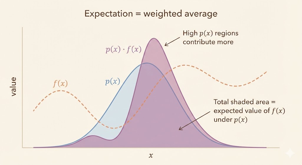
A generic expectation can be written as \[ s = \sum_x p(x) f(x) = \mathbb{E}_p[f(x)] \quad \text{or} \quad s = \int p(x) f(x) \, dx. \]
Monte Carlo replaces the expectation with an empirical mean: \[ \hat{s} = \frac{1}{n} \sum_{i=1}^n f\bigl(x^{(i)}\bigr), \quad x^{(i)} \sim p(x). \] By the law of large numbers, as \(n \to \infty\) the estimate converges to the true expectation. The estimator is unbiased when the samples are independent and identically distributed, and its typical error scales like \(O(1/\sqrt{n})\).
Dice example
For a fair die \(X \in \{1,2,3,4,5,6\}\) with \(p(x)=1/6\), \[ \begin{aligned} \mathbb{E}[X] &= \sum_x x p(x) \\ &= \frac{1}{6} + \frac{2}{6} + \frac{3}{6} + \frac{4}{6} + \frac{5}{6} + \frac{6}{6} \\ &= 3.5. \end{aligned} \] Expanded sum: \(\frac{1}{6} + \frac{2}{6} + \frac{3}{6} + \frac{4}{6} + \frac{5}{6} + \frac{6}{6} = 3.5\).
Sampling \(x^{(1)},\dots,x^{(n)}\) from \(p(x)\) gives \[ \hat{\mu} = \frac{1}{n}\sum_{i=1}^n x^{(i)}, \] which approaches 3.5 as \(n\) grows. In practice, this is just the average of \(n\) dice rolls, and the law of large numbers guarantees it concentrates near 3.5.
Variance scaling
The variance of a Monte Carlo estimator decreases like \(1/n\): \[ \mathrm{Var}[\hat{s}] = \frac{1}{n^2} \sum_{i=1}^n \mathrm{Var}[f(x)] = \frac{\mathrm{Var}[f(x)]}{n}. \] More samples reduce noise, but each extra digit of accuracy costs exponentially more samples.
Importance sampling
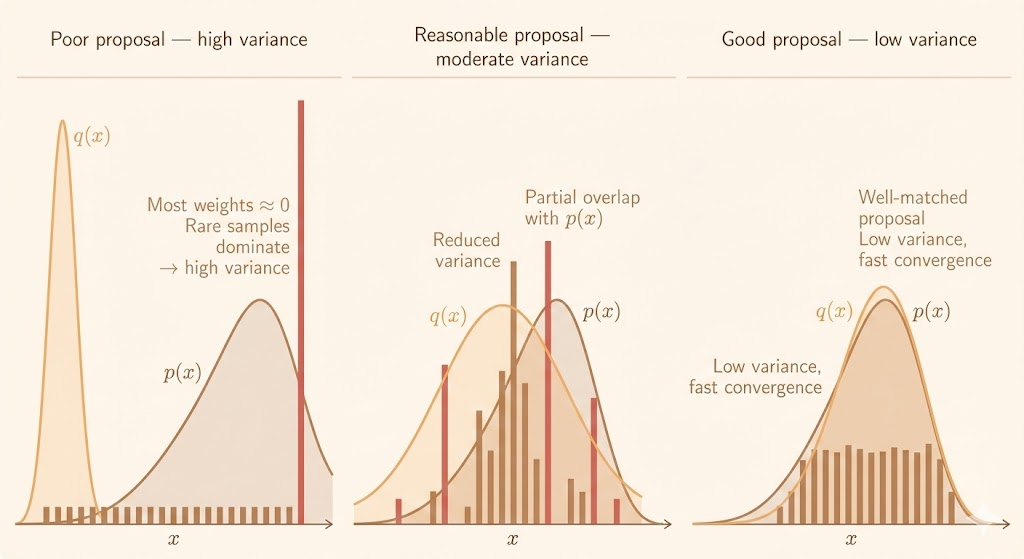
When sampling directly from \(p(x)\) is difficult, importance sampling draws samples from a proposal \(q(x)\) and reweights them: \[ \mathbb{E}_p[f(x)] = \mathbb{E}_q\left[f(x) \frac{p(x)}{q(x)}\right]. \] The proposal \(q(x)\) should be easy to sample from and should cover the support of \(p(x)\). If \(q\) puts too little mass where \(p\) is large, the weights explode and variance becomes unstable.
A practical estimator is \[ \hat{s} = \frac{1}{n}\sum_{i=1}^n f(x^{(i)})\,\frac{p(x^{(i)})}{q(x^{(i)})}, \quad x^{(i)} \sim q(x). \] The estimator stays unbiased, but the variance depends on how well \(q(x)\) matches \(p(x)\). Poor proposals create extreme weights and high variance; good proposals concentrate mass where \(p(x)\) is large and reduce variance dramatically.
Markov chains
When neither direct sampling nor a good proposal is available, Markov chains provide a way to generate dependent samples. A Markov chain uses a transition operator \[ x^{(t+1)} \sim T(x^{(t+1)} \mid x^{(t)}), \] so the next state depends only on the current state (the Markov property). The samples are correlated, but they can still be used once the chain has mixed and reached its stationary distribution.
Distribution dynamics
Let \(q^{(t)}(x)\) be the distribution at step \(t\). The evolution is \[ q^{(t+1)}(x') = \sum_x q^{(t)}(x)\, T(x'\mid x), \] or in matrix form \(\mathbf{q}^{(t+1)} = A\mathbf{q}^{(t)}\), where \(A\) is a stochastic transition matrix whose columns sum to 1.
Stationary distribution
Under mild conditions (irreducibility and aperiodicity), the chain converges to a stationary distribution \(q^*\): \[ q^* = A q^*. \] If \(q^* = p(x)\), then long-run samples approximate the target distribution. In practice we discard an initial burn-in period and then use the correlated samples for estimation. This is the foundation of Markov Chain Monte Carlo (MCMC), especially for energy-based models where the normalization constant is unknown.
Gibbs sampling
Gibbs sampling updates one variable (or a block of variables) at a time using its conditional distribution given all others: \[ x_i^{(t+1)} \sim p(x_i \mid x_{-i}^{(t)}). \] Cycling through all variables defines a Markov chain whose stationary distribution matches the target model \(p_{\text{model}}(x)\), making it effective for undirected graphical models and energy-based models such as RBMs. It is simple to implement when the conditionals are easy to sample.
Mixing and tempering
MCMC can mix slowly when the target distribution is multimodal. Local transitions tend to stay within one mode, yielding highly correlated samples and slow exploration of the full support. This behavior is often described as noisy gradient descent on the energy landscape, where moving between modes requires climbing energy barriers.
Tempering introduces a temperature parameter: \[ p_\beta(x) \propto \exp(-\beta E(x)). \] Lower \(\beta\) (higher temperature) flattens the energy landscape and improves mixing; higher \(\beta\) yields more accurate samples. Parallel tempering and tempered transitions run chains at multiple temperatures, allowing high-temperature chains to explore while low-temperature chains retain fidelity.
Empirically, deep representations can improve mixing because the latent space is often smoother and less multimodal than the original data space, making transitions between modes more likely.
Summary
Monte Carlo methods replace intractable expectations with sample averages, trade accuracy for computation, and rely on variance reduction strategies to be practical. Importance sampling improves efficiency when a good proposal is available, while MCMC methods like Gibbs sampling handle cases where only local transitions are feasible.