Lecture 11: Minimize ||x|| subject to Ax=b
When solving constrained optimization problems of the form minimize \(\|x\|\) subject to \(Ax = b\), the choice of norm fundamentally changes the geometry of the solution and its properties. This lecture explores how different norms lead to different biases: sparsity (L1), smoothness (L2), or balance (L∞).
Three Norms and Their Geometric Intuition
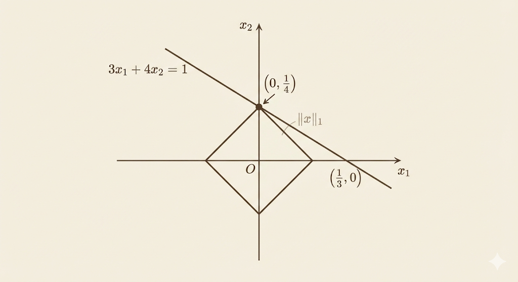
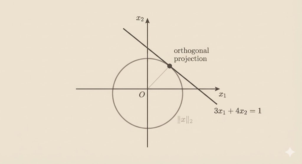
Consider the simple real case: \(3x_1 + 4x_2 = 1\). The constraint defines a line in 2D. As we expand a norm ball from the origin, it will eventually touch this line. The first contact point is the minimum-norm solution.
L1 Norm: Sparsity
\[\|x\|_1 = |x_1| + |x_2|\]
The L1 norm ball is a diamond (rotated square). As the diamond expands, it touches the constraint line at a corner:
\[x^* = \left(0, \frac{1}{4}\right)\]
Key insight: Because the diamond has sharp corners aligned with coordinate axes, optimal solutions tend to lie at these corners—setting some components exactly to zero. L1 minimization promotes sparsity, which is why it’s used in compressed sensing and sparse recovery.
L2 Norm: Smoothness
\[\|x\|_2 = \sqrt{x_1^2 + x_2^2}\]
The L2 norm ball is a circle. It touches the constraint line smoothly at a point of tangency:
\[x^* = \left(\frac{3}{25}, \frac{4}{25}\right)\]
This optimal point lies in the direction of the normal vector \(\mathbf{n} = \begin{bmatrix} 3 \\ 4 \end{bmatrix}\) of the constraint line. L2 minimization is isotropic—it doesn’t favor sparsity or equal components, instead finding the orthogonal projection of the origin onto the constraint surface.
L∞ Norm: Balance
\[\|x\|_\infty = \max(|x_1|, |x_2|)\]
The L∞ norm ball is an axis-aligned square. It first touches the constraint line where the two components are equal:
\[x_1 = x_2 \quad \Rightarrow \quad 7x_1 = 1 \quad \Rightarrow \quad x_1 = x_2 = \frac{1}{7}\]
L∞ minimization tends to balance parameters, equalizing the magnitudes of components.
Comparison Table
| Norm | Norm Ball | First Contact | Induced Bias |
|---|---|---|---|
| \(L_1\) | Diamond | Corner | Sparsity: zeros out some components |
| \(L_2\) | Circle | Smooth tangency | Smoothness: aligned with normal direction |
| \(L_∞\) | Square | Vertex or edge | Balance: equalizes component magnitudes |
QR Factorization and Minimum-Norm Solutions
When \(A\) has full column rank, the minimum-norm solution \(x^*\) can be computed via QR factorization: \(A = QR\).
Gram–Schmidt Orthogonalization
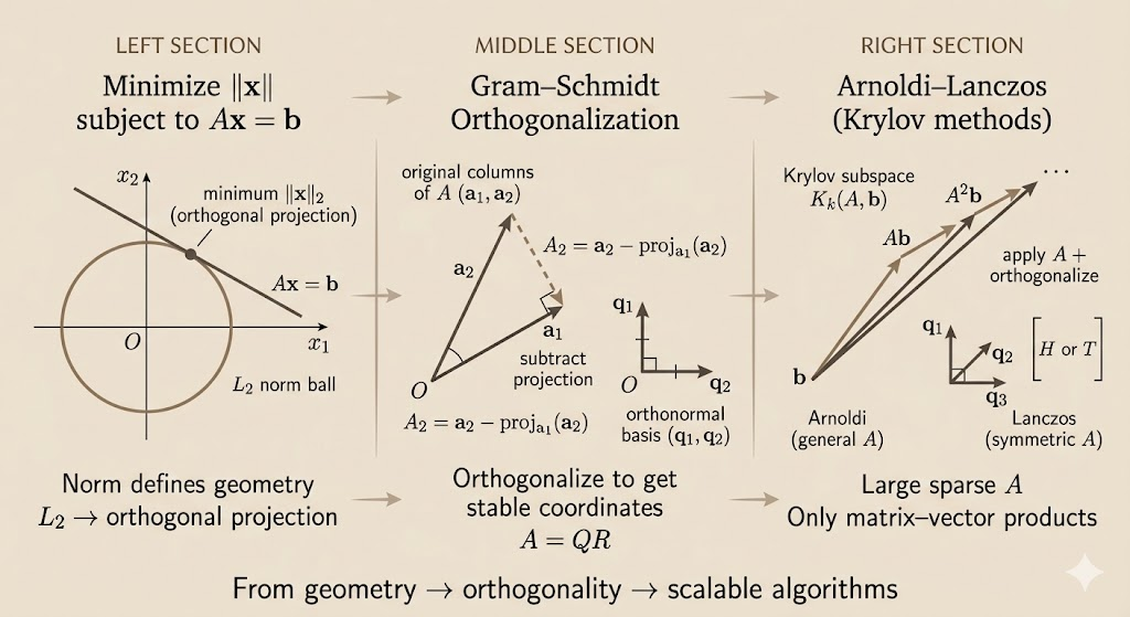
Gram–Schmidt is a procedure that converts the columns of \(A\) into an orthonormal basis:
\[q_1 = \frac{a_1}{\|a_1\|_2}, \quad q_k = \frac{a_k - \sum_{i=1}^{k-1} (a_k^\top q_i) q_i}{\left\|a_k - \sum_{i=1}^{k-1} (a_k^\top q_i) q_i\right\|_2}\]
The resulting orthonormal matrix \(Q\) and upper-triangular matrix \(R\) satisfy:
\[A = QR\]
For the least-squares problem \(\min \|Ax - b\|_2^2\), the minimum-norm solution is:
\[x^* = A^\dagger b = R^{-1} Q^\top b\]
where \(A^\dagger\) is the pseudoinverse.
Numerical Stability: Column Pivoting
When columns of \(A\) are nearly linearly dependent, standard Gram–Schmidt becomes numerically unstable, producing very small pivots and large coefficients.
Column pivoting mitigates this by selecting at each step the column with the largest remaining norm as the next pivot, rather than following the original column order.
Example: Given nearly dependent columns: \[a_1 = \begin{bmatrix}1\\1\\1\end{bmatrix}, \quad a_2 = \begin{bmatrix}1\\1\\1+\varepsilon\end{bmatrix}, \quad a_3 = \begin{bmatrix}0\\1\\0\end{bmatrix}, \quad \varepsilon = 10^{-6}\]
Column pivoting selects \(a_3\) after \(a_1\) because its remaining norm (after projecting out the \(a_1\) component) is much larger than that of \(a_2\). This preserves numerical stability.
Krylov Subspace Methods
For large, sparse matrices \(A\), direct factorization (QR or SVD) is computationally prohibitive. Instead, we restrict the search to a low-dimensional Krylov subspace.
The Krylov Subspace
The Krylov subspace of dimension \(k\) is defined as:
\[\mathcal{K}_k(A, b) = \text{span}\{b, Ab, A^2b, \ldots, A^{k-1}b\}\]
The approximate solution is then constrained to lie in this space:
\[x_k \in \mathcal{K}_k(A, b)\]
Key advantage: Constructing the Krylov subspace requires only matrix–vector products, which are highly efficient for sparse matrices.
Arnoldi–Lanczos: Orthogonalization in Krylov Space
The vectors \(b, Ab, A^2b, \ldots\) quickly become nearly linearly dependent. Gram–Schmidt is applied to orthogonalize these vectors, producing a numerically stable orthonormal basis for the Krylov subspace.
This is the foundation of iterative solvers like: - GMRES (General Minimum Residual) for non-symmetric \(A\) - Lanczos for symmetric \(A\)
Both methods maintain orthogonal bases within the Krylov subspace, enabling efficient approximation of solutions to \(Ax = b\) without forming or factorizing \(A\) explicitly.
Key Insight
The choice of norm determines the geometric bias of the solution. L1 prefers sparsity (corners), L2 prefers smoothness (tangency), and L∞ prefers balance. For large-scale problems, Krylov methods exploit the structure of the matrix by restricting the search to low-dimensional subspaces, using iterative Gram–Schmidt to maintain numerical stability. The interplay between geometry (norms), algebra (QR factorization), and numerics (pivoting, Krylov methods) is central to modern computational linear algebra.