Goodfellow Deep Learning — Chapter 19: Approximate Inference
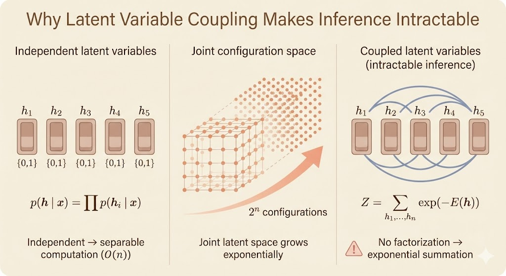
Exact inference in deep latent variable models is usually intractable. The issue is not just the size of the latent space, but the coupling between latent variables that destroys factorization. As a result, marginalizing over all configurations scales exponentially.
Why inference becomes intractable
If latent variables are conditionally independent, inference can exploit factorization and reduce exponential sums to linear-time message passing. When latents are coupled, the posterior requires summing or integrating over all joint configurations, which scales as \(O(2^n)\) for binary latents.
Inference as optimization (ELBO)
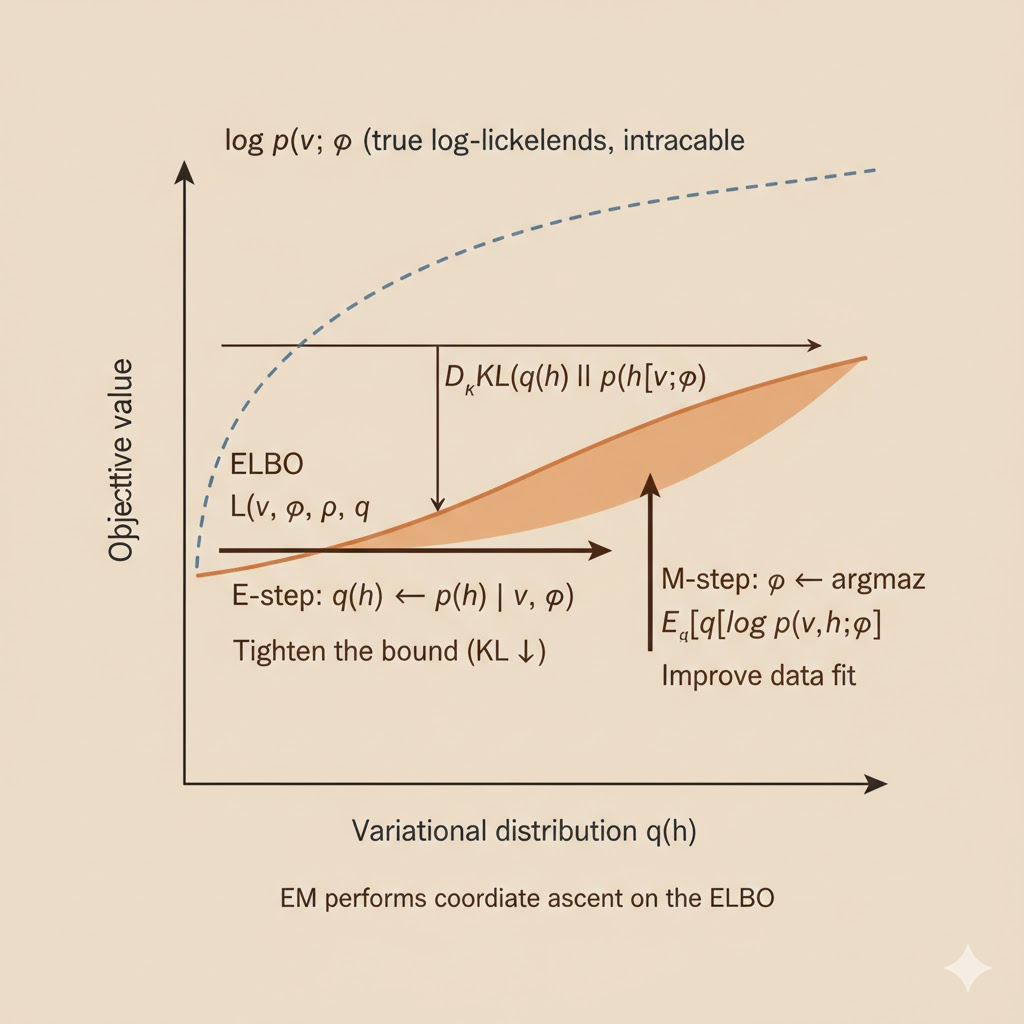
When the exact marginal likelihood \(\log p(v;\theta)\) is hard to compute, we optimize a lower bound instead. For any distribution \(q(h)\), \[ \log p(v;\theta) = \mathcal{L}(v,\theta,q) + D_{\mathrm{KL}}\big(q(h)\,\|\,p(h\mid v;\theta)\big), \] so \[ \mathcal{L}(v,\theta,q) \le \log p(v;\theta). \] Expanding the bound gives \[ \mathcal{L}(v,\theta,q) = \mathbb{E}_q[\log p(v,h;\theta)] + H(q), \] where \(H(q)=-\mathbb{E}_q[\log q(h)]\) is the entropy. The ELBO trades exact marginalization for a tractable optimization problem over \(q\).
Expectation-Maximization (EM)
EM performs coordinate ascent on the ELBO:
E-step (inference). With \(\theta\) fixed, set \[ q(h)=p(h\mid v;\theta), \] which minimizes the KL divergence to the true posterior.
M-step (learning). With \(q\) fixed, update parameters by maximizing the expected complete-data log-likelihood \[ \mathbb{E}_{q(h)}[\log p(v,h;\theta)]. \] Each iteration increases the data log-likelihood without explicitly summing over all latent configurations.
MAP inference and sparse coding
MAP inference replaces the full posterior with a single most likely configuration: \[ h^* = \arg\max_h p(h\mid v). \] Variationally, this corresponds to restricting \(q(h)\) to a Dirac delta distribution \(\delta(h-\mu)\), which yields \[ \mu^* = \arg\max_{\mu} \log p(h=\mu, v). \]
Sparse coding is a classic example. With a Laplace prior \(p(h_i)\propto \exp(-\lambda|h_i|)\) and a linear generative model, MAP inference becomes the convex problem \[ \min_h \; \|v-Wh\|_2^2 + \lambda\|h\|_1. \] This turns probabilistic inference into deterministic optimization.
Variational inference and mean-field
Variational inference replaces the intractable posterior with a tractable family. A common choice is mean-field: \[ q(h\mid v)=\prod_i q(h_i\mid v). \] The optimal factors satisfy the fixed-point update \[ q_i(h_i\mid v) \propto \exp\Big(\mathbb{E}_{q_{-i}}[\log p(v,h)]\Big), \] which yields iterative inference updates. For continuous latent variables in linear-Gaussian models, the optimal \(q(h)\) is Gaussian; for discrete latents, the updates reduce to coordinate-wise optimization of the ELBO.