Batch Normalization: Accelerating Deep Network Training
Paper: Batch Normalization: Accelerating Deep Network Training by Reducing Internal Covariate Shift
Problem
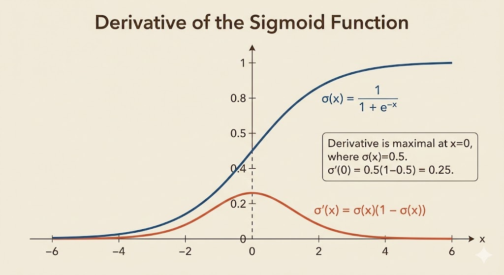
Deep networks train slowly because the distribution of activations keeps shifting as earlier layers change. This pushes activations into saturated regions (e.g., sigmoid), where gradients vanish and optimization stalls.
For a sigmoid \(g(x)=\frac{1}{1+e^{-x}}\), as \(|x|\) grows, \(g'(x)\to 0\). If the pre-activation \(x=Wu+b\) drifts, gradients to \(u\) shrink and learning slows.
Key idea
Normalize activations within each mini-batch to stabilize their distribution, then allow the model to restore scale and shift with learnable parameters.
Intuition: BN keeps each feature in a predictable range so later layers do not chase a moving target, while \(\gamma,\beta\) preserve expressiveness by letting the network undo normalization if needed.
Why normalization must be differentiable
If we normalize using batch statistics but ignore them in backprop, the update can be canceled by the next normalization step.
Example: \(\hat{x}=x-\mathbb{E}(x)\). If we update \(b\) without accounting for \(\mathbb{E}(x)\), the next recomputed mean removes that update. So the normalization must be part of the computation graph.
Where BN is applied
For a layer pre-activation \(z = Wx + b\), the paper applies BN to \(z\) before the nonlinearity:
\[ \tilde{z} = \text{BN}(z), \quad y = \phi(\tilde{z}) \]
Some modern implementations apply BN after the activation; the key is normalizing each feature (or channel) consistently.
BatchNorm for a vector layer
For a mini-batch \(\mathcal{B} = \{x_1,\dots,x_m\}\):
\[ \mu_\mathcal{B} = \frac{1}{m}\sum_{i=1}^m x_i,\quad \sigma^2_\mathcal{B} = \frac{1}{m}\sum_{i=1}^m (x_i-\mu_\mathcal{B})^2 \]
Normalize and re-scale:
\[ \hat{x}_i = \frac{x_i-\mu_\mathcal{B}}{\sqrt{\sigma^2_\mathcal{B}+\epsilon}},\quad y_i = \gamma\hat{x}_i + \beta \]
- \(\gamma,\beta\) are learnable, so the layer can recover the original activation scale if needed.
Gradients (core idea)
BatchNorm is fully differentiable:
- \(\frac{\partial L}{\partial \hat{x}_i} = \frac{\partial L}{\partial y_i}\cdot \gamma\)
- \(\frac{\partial L}{\partial \gamma} = \sum_i \frac{\partial L}{\partial y_i}\hat{x}_i\)
- \(\frac{\partial L}{\partial \beta} = \sum_i \frac{\partial L}{\partial y_i}\)
2D BatchNorm (CNNs)
For \(x\in\mathbb{R}^{N\times C\times H\times W}\), normalize per channel:
\[ \mu_c = \frac{1}{NHW}\sum_{i,h,w} x_{i,c,h,w},\quad \sigma_c^2 = \frac{1}{NHW}\sum_{i,h,w} (x_{i,c,h,w}-\mu_c)^2 \]
\[ \hat{x}_{i,c,h,w} = \frac{x_{i,c,h,w}-\mu_c}{\sqrt{\sigma_c^2+\epsilon}},\quad y_{i,c,h,w} = \gamma_c\hat{x}_{i,c,h,w}+\beta_c \]
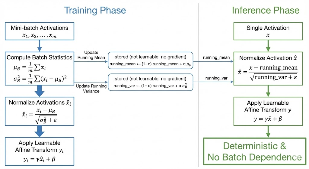
Training vs inference
- Training uses batch statistics.
- Inference uses running averages of mean/variance accumulated during training.
A typical update for running stats:
\[ \mu_{\text{run}} \leftarrow \rho\,\mu_{\text{run}} + (1-\rho)\,\mu_{\mathcal{B}},\quad \sigma^2_{\text{run}} \leftarrow \rho\,\sigma^2_{\text{run}} + (1-\rho)\,\sigma^2_{\mathcal{B}} \]
This makes predictions deterministic and independent of batch composition.
Effects and practical notes
- Enables larger learning rates and faster convergence.
- Acts as a form of regularization (mini-batch noise).
- Reduces sensitivity to initialization.
- Improves conditioning by keeping feature scales comparable.
Takeaway. BatchNorm stabilizes activation distributions by normalizing per mini-batch and then re-introducing scale and shift. This makes deep optimization easier and faster while adding mild regularization.