Transformer: Attention Is All You Need
Paper: Attention Is All You Need
Previous neural sequence models treated language as a temporal process, relying on recurrence or convolution to propagate information step by step. Attention was introduced to assist these architectures, but remained a secondary mechanism.
The Transformer redefines this formulation. Instead of modeling sequences through recursion, it treats them as sets of interacting elements and relies entirely on attention to capture dependencies. By eliminating recurrence, the Transformer enables parallel computation and marks a fundamental shift in sequence modeling.
Model Architecture
Tokens Embedding and Position Encoding
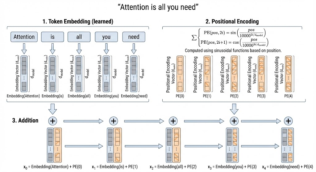
The input sequence is first tokenized into discrete tokens. Each token index is mapped to a continuous vector through a learned embedding matrix, producing a representation in \(d_{model}\) dimensions for each token.
Since the Transformer operates entirely on vector representations, token embeddings are the basic units processed by the model. However, unlike recurrent or convolutional architectures, the Transformer itself has no inherent notion of token order. To inject order information, positional encoding is added to each token embedding. The positional encoding has the same dimensionality as the token embedding, so they can be combined by element-wise addition before entering subsequent Transformer layers.
In the original paper, positional encoding is fixed sinusoidal (not learned): \[ PE(pos,2i)=\sin\left(\frac{pos}{10000^{2i/d_{model}}}\right), \] \[ PE(pos,2i+1)=\cos\left(\frac{pos}{10000^{2i/d_{model}}}\right). \]
The input at position \(pos\) becomes: \[ x_{pos}=\text{Embedding}(x_{pos})+PE(pos). \]

Encoder and Decoder
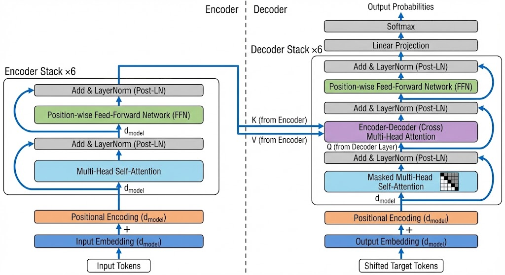
The original model uses a stack of 6 encoder layers and 6 decoder layers.
Encoder
Each encoder layer contains:
- A multi-head self-attention sublayer
- A position-wise fully connected feed-forward sublayer
Each sublayer is wrapped by residual connection followed by layer normalization: \[ \text{LayerNorm}(x + \text{Sublayer}(x)). \]
Decoder
Each decoder layer contains:
- A masked multi-head self-attention sublayer
- An encoder-decoder multi-head attention sublayer
- A position-wise fully connected feed-forward sublayer
In encoder-decoder attention:
- Queries come from decoder states
- Keys and values come from encoder outputs
Each decoder sublayer also uses residual connection + layer normalization.

Scaled Dot-Product Attention
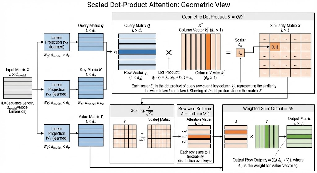
Single-head form: \[ \text{Attention}(Q,K,V)=\text{softmax}\left(\frac{QK^\top}{\sqrt{d_k}}\right)V. \] For the special case \(d_k=d_{model}\), the denominator can be written as \(\sqrt{d_{model}}\).
Given input representation \(X \in \mathbb{R}^{L \times d_{model}}\): \[ Q = XW_Q, \quad K = XW_K, \quad V = XW_V. \] where \(W_Q, W_K, W_V\) are learned projection matrices.
Shapes:
- \(Q, K \in \mathbb{R}^{L \times d_k}\)
- \(V \in \mathbb{R}^{L \times d_v}\)
Step 1: Compute attention scores \[ S=QK^\top \in \mathbb{R}^{L \times L} \] where \(S_{ij}\) measures similarity between token \(i\) and token \(j\).
Step 2: Scale \[ S=\frac{QK^\top}{\sqrt{d_k}}. \] Scaling prevents dot products from becoming too large and saturating softmax.
Step 3: Apply row-wise softmax \[ A=\text{softmax}(S). \] Each row of \(A\) sums to 1.
Step 4: Weighted sum over values \[ \text{Output}=AV \in \mathbb{R}^{L \times d_v}. \] Each output row is a weighted combination of value vectors.

Multi-Head Attention
Instead of one attention head, Transformer projects \(Q,K,V\) into \(h\) different subspaces and runs attention in parallel: \[ \text{head}_i=\text{Attention}(XW_i^Q, XW_i^K, XW_i^V), \] \[ \text{MultiHead}(Q,K,V)=\text{Concat}(\text{head}_1,\dots,\text{head}_h)W^O. \]
Where:
- \(W_i^Q \in \mathbb{R}^{d_{model}\times d_k}\)
- \(W_i^K \in \mathbb{R}^{d_{model}\times d_k}\)
- \(W_i^V \in \mathbb{R}^{d_{model}\times d_v}\)
- \(W^O \in \mathbb{R}^{(h\cdot d_v)\times d_{model}}\)
This lets different heads capture different relations and then combine them back into \(d_{model}\) space.
Takeaway. Attention moved from an auxiliary mechanism to the core sequence operator, enabling fully parallel Transformer training.