MIT 18.065: Lecture 19 - Saddle Point and the Max–Min Principle
Saddle point of the Rayleigh quotient
For a symmetric matrix \(S\), the Rayleigh quotient is \[ R(x)=\frac{x^\top S x}{x^\top x}. \] A standard derivative identity gives \[ \nabla_x (x^\top S x) = (S+S^\top)x = 2Sx,\qquad \nabla_x (x^\top x)=2x. \] Applying the quotient rule yields \[ \nabla R(x)=\frac{2}{x^\top x}\Big(Sx-\frac{x^\top S x}{x^\top x}x\Big). \] Therefore, every stationary point satisfies \[ Sx = R(x)x, \] so stationary points are exactly the eigenvectors of \(S\), and the stationary values are the eigenvalues.
Example: diagonal matrix
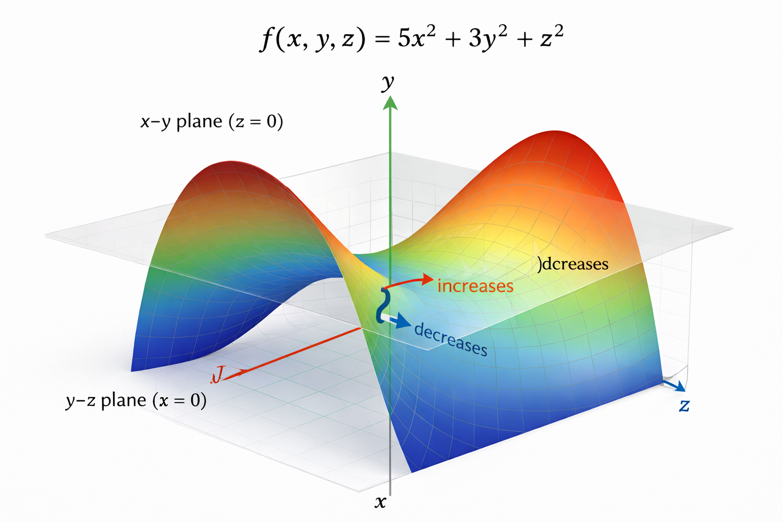
Let \[ S=\begin{bmatrix} 5&0&0\\ 0&3&0\\ 0&0&1 \end{bmatrix},\qquad x=\begin{bmatrix}u\\v\\w\end{bmatrix}. \] Then \[ R(x)=\frac{5u^2+3v^2+w^2}{u^2+v^2+w^2}. \] The eigenvectors are the coordinate axes:
- \(\lambda_1=5\) at \(x=e_1\) is the global maximum of \(R(x)\).
- \(\lambda_3=1\) at \(x=e_3\) is the global minimum of \(R(x)\).
- \(\lambda_2=3\) at \(x=e_2\) is a saddle: the gradient vanishes, but nearby directions increase or decrease \(R(x)\).
The max–min principle (Courant–Fischer)
For a symmetric matrix \(A\) with eigenvalues \[ \lambda_1\ge \lambda_2\ge \dots\ge \lambda_n, \] the Rayleigh quotient satisfies \[ \lambda_k=\max_{\dim V=k}\;\min_{x\in V} R(x). \] Interpretation:
- Choose a \(k\)-dimensional subspace \(V\).
- Inside that subspace, the smallest Rayleigh quotient is a “worst case.”
- Among all \(k\)-dimensional subspaces, pick the one that makes this worst case as large as possible.
That optimal worst-case value is exactly \(\lambda_k\). So:
- \(\lambda_1\) is the global maximum of \(R(x)\).
- \(\lambda_n\) is the global minimum.
- Intermediate eigenvalues are saddle values: max–min values of restricted problems.
Polynomial interpolation and overfitting
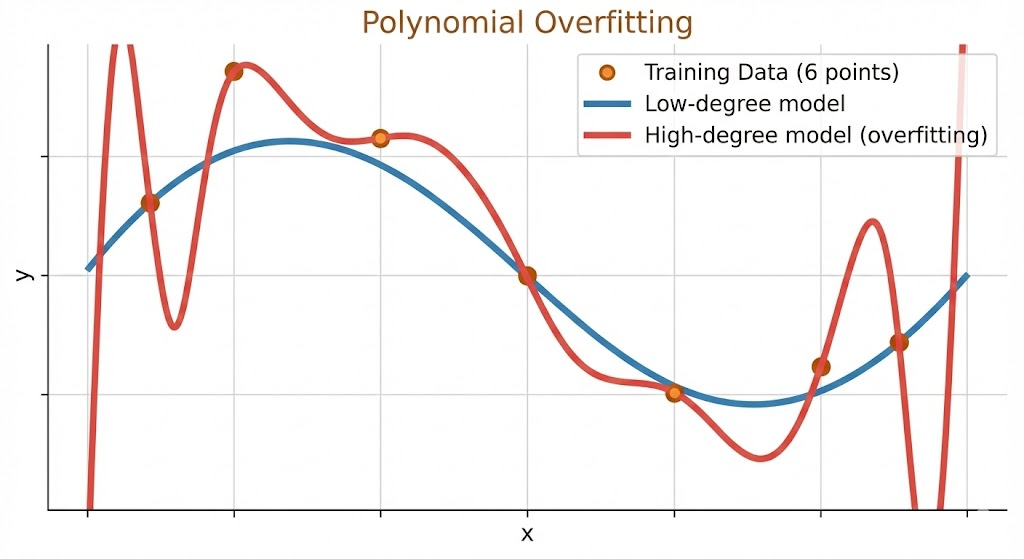
Given \(N\) distinct data points \((x_i,y_i)\), there exists a unique polynomial of degree at most \(N-1\), \[ p(x)=c_0+c_1x+\dots+c_{N-1}x^{N-1}, \] that interpolates all points: \(p(x_i)=y_i\).
Special cases:
- Degree 0 fits 1 point
- Degree 1 fits 2 points
- Degree 2 fits 3 points
- Degree \(N-1\) fits \(N\) points
Overfitting perspective. Exact interpolation can oscillate wildly between points, so perfect training fit does not guarantee good generalization.
Variance, covariance, and joint probability
Probability basics
Discrete distribution: \[ \sum_{i=1}^n p_i=1. \] Continuous distribution: \[ \int_{-\infty}^{\infty} p(x)\,dx=1. \]
Mean and variance
Sample mean: \[ \mu=\frac{1}{N}\sum_{i=1}^N x_i. \] Expected value: \[ E[X]=\sum_{i=1}^n p_i x_i\quad\text{or}\quad E[X]=\int x\,p(x)\,dx. \] Sample variance: \[ \frac{1}{N-1}\sum_{i=1}^N (x_i-\mu)^2. \] Variance: \[ \mathrm{Var}(X)=E[(X-E[X])^2]. \]
Covariance and dependence
Covariance measures linear dependence: \[ \mathrm{Cov}(X,Y)=E[(X-E[X])(Y-E[Y])]. \]
- Independent variables: \(\mathrm{Cov}(X,Y)=0\).
- Perfect dependence (one variable determines the other): covariance is maximized in magnitude.
Intuition from coin flips and polling:
- Two unrelated coin flips are independent, so covariance is 0.
- Two “glued” coins always match, giving maximal covariance.
- Family members in a poll are correlated but not identical: covariance is positive but not maximal.
Takeaway. The Rayleigh quotient links eigenvalues to max–min geometry. Its stationary points are eigenvectors, and intermediate eigenvalues are saddle values. The same “fit vs. generalize” tension appears in high‑degree interpolation, while variance and covariance quantify how randomness and dependence shape data.