Gilbert Strang’s Calculus: Big Picture Integral
Integrals and derivatives can be mostly explained by working (very briefly) with sums and differences.
- Gilbert Strang
The connection between two functions
The key connection is between a height/distance function and a slope function. This pair is a two-way map: derivative gives local change from total accumulation, and integral rebuilds total accumulation from local change (up to an initial value).
- Height/Distance function: \(y(x)\)
This function represents accumulated height or distance. - Slope function: \[ s(x)=\frac{dy}{dx}=\lim_{\Delta x\to 0}\frac{\Delta y}{\Delta x} \] This function represents the instantaneous rate of change (for distance-time, this is speed).
Examples:
- If \(y=x^n\), then \(\frac{dy}{dx}=nx^{n-1}\).
- If \(\frac{dy}{dx}=x^n\), then \[ y(x)=\frac{x^{n+1}}{n+1}+C. \]
From slope to distance
Suppose we know the slope each hour and want distance back.
Hourly slopes: \[ 4,\ 3,\ 2,\ 1,\ 0. \]
Cumulative distance:
- Hour 1: \(4\)
- Hour 2: \(4+3=7\)
- Hour 3: \(7+2=9\)
- Hour 4: \(9+1=10\)
- Hour 5: \(10+0=10\)
From an algebra view, sample distance at times as \(y_0,y_1,y_2,\dots,y_n\). Then each increment is: \[ \Delta y_k=y_k-y_{k-1}. \] Summing all increments gives: \[ \sum_{k=1}^n \Delta y_k =(y_1-y_0)+(y_2-y_1)+\cdots+(y_n-y_{n-1}) =y_n-y_0. \]
This is exactly “final value minus initial value.”
Another equivalent form is: \[ \sum \left(\frac{\Delta y}{\Delta x}\right)\Delta x = y_{\text{last}}-y_{\text{first}}. \]
As \(\Delta x\) gets smaller and smaller, \(\frac{\Delta y}{\Delta x}\) approaches the slope function \(\frac{dy}{dx}\).
The answer is as simple as changing \(\sum\) to \(\int\):
\[ \int s(x)\,dx. \]
Here \(s(x)\) is the slope, and \(dx\) is an infinitesimal change in \(x\). Geometrically, this is accumulated area under the slope curve.
Example
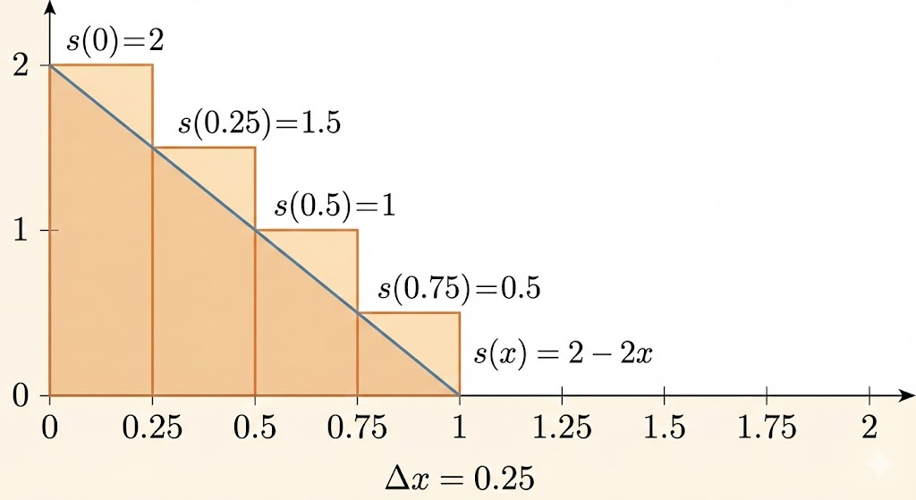
Slope function: \[ s(x)=2-2x. \]
This starts at 2 (when \(x=0\)) and drops to 0 (when \(x=1\)). To get height/distance, we can first look at a discrete approximation, then the integral limit.
Discrete point of view
Split \([0,1]\) into 4 equal intervals, so \(\Delta x=\frac14\). Use left endpoints as piecewise-constant speeds.
Speeds at left endpoints:
- \(x=0\): \(2\)
- \(x=\frac14\): \(1.5\)
- \(x=\frac12\): \(1\)
- \(x=\frac34\): \(0.5\)
Left Riemann sum: \[ 2\Delta x+1.5\Delta x+1\Delta x+0.5\Delta x =5\Delta x=\frac54=1.25. \]
Observation:
- Inside each interval, slope is decreasing.
- Using the left endpoint gives a larger rectangle than the true area.
- So this is an overestimate.
Now use smaller intervals, for example \(\Delta x=\frac18\): \[ 2\Delta x+1.75\Delta x+1.5\Delta x+1.25\Delta x+1\Delta x+0.75\Delta x+0.5\Delta x+0.25\Delta x =9\Delta x=\frac98=1.125. \]
The estimate gets closer as \(\Delta x\to 0\).
Integral point of view
From the discrete view, smaller \(\Delta x\) gives better accuracy. In the limit, rectangles become infinitesimally thin, and the sum becomes the exact area: \[ \int_0^x (2-2t)\,dt. \]
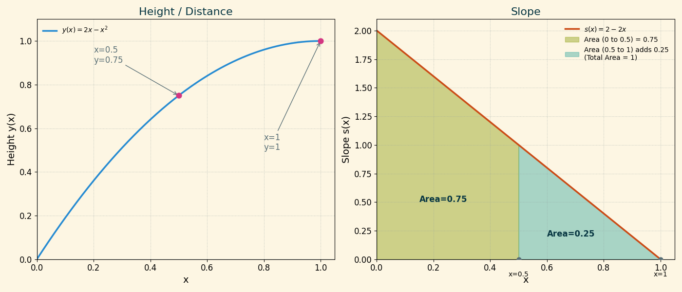
Areas:
- At \(x=1\): area is triangle area \[ \frac{1\cdot 2}{2}=1. \]
- At \(x=0.5\): area can be computed either as
- big triangle minus small triangle, or
- trapezoid area from \(x=0\) to \(x=0.5\).
Both give \(0.75\).
Proof
Find an antiderivative of \(s(x)=2-2x\): \[ y(x)=2x-x^2+C. \] If we set \(y(0)=0\), then \(C=0\), so \[ y(x)=2x-x^2. \]
Check:
- \(x=1\): \(y(1)=2(1)-1^2=1\)
- \(x=0.5\): \(y(0.5)=2(0.5)-(0.5)^2=1-0.25=0.75\)
So the integral view and algebraic antiderivative match exactly.