MIT 18.065: Lecture 20 - Probability Definitions and Inequalities
Variance identity
Variance can be written in a compact and useful form: \[ \mathrm{Var}(X)=E[(X-m)^2]=E[X^2]-m^2,\quad m=E[X]. \]
For a discrete variable with values \(x_i\) and probabilities \(p_i\): \[ \sum_{i=1}^n p_i(x_i-m)^2 =\sum_{i=1}^n p_i x_i^2 -2m\sum_{i=1}^n p_i x_i + m^2\sum_{i=1}^n p_i. \] Using \[ \sum_{i=1}^n p_i x_i = m,\qquad \sum_{i=1}^n p_i=1, \] we get \[ \mathrm{Var}(X)=E[X^2]-m^2=E[X^2]-(E[X])^2. \]
Markov’s inequality
If \(X\ge 0\) and \(a>0\), then \[ \Pr(X\ge a)\le \frac{E[X]}{a}. \]
Example
Suppose \(E[X]=1\) and \(a=3\) for a nonnegative discrete variable taking values in \(\{1,2,3,4,5\}\). Write \[ 1=\sum_{i=1}^5 i\,p_i =1p_1+2p_2+3(p_3+p_4+p_5)+(p_4+2p_5). \] Since all probabilities are nonnegative, the last two terms are \(\ge 0\), so \[ 3(p_3+p_4+p_5)\le 1 \;\Rightarrow\; p_3+p_4+p_5\le \frac13. \] Therefore, \[ \Pr(X\ge 3)\le \frac13, \] which matches Markov: \[ \Pr(X\ge 3)\le \frac{E[X]}{3}=\frac13. \]
Chebyshev’s inequality
Chebyshev follows directly by applying Markov to \[ Y=(X-m)^2\ge 0. \] Then \[ E[Y]=E[(X-m)^2]=\sigma^2,\qquad \{|X-m|\ge a\}=\{(X-m)^2\ge a^2\}. \] So \[ \Pr(|X-m|\ge a)=\Pr((X-m)^2\ge a^2)\le \frac{\sigma^2}{a^2}. \]
Joint probability
For two independent fair coins \((C_1,C_2)\), the joint table is \[ \begin{array}{c|cc} & C_2=H & C_2=T\\ \hline C_1=H & 0.25 & 0.25\\ C_1=T & 0.25 & 0.25 \end{array} \]
If the two coins are “glued” (always same face), the joint table becomes \[ \begin{array}{c|cc} & C_2=H & C_2=T\\ \hline C_1=H & 0.5 & 0\\ C_1=T & 0 & 0.5 \end{array} \]
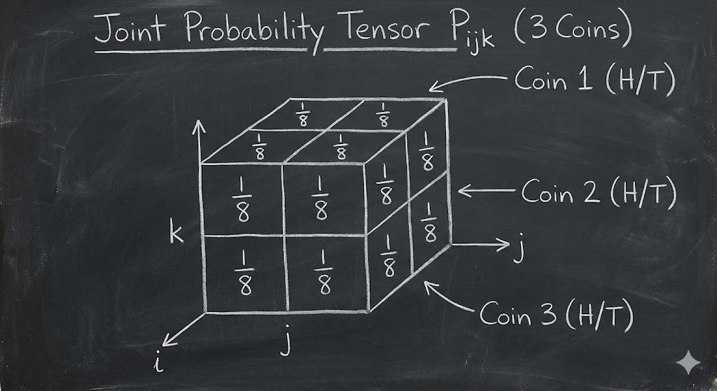
For three random variables, the joint distribution is a third-order tensor: \[ P_{ijk}=\Pr(X_1=i,X_2=j,X_3=k). \]
Marginals come from summing over axes. For example: \[ P_j=\sum_i P_{ij}. \]
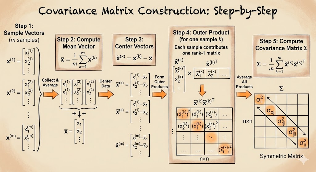
Covariance matrix
Let \[ X=\begin{bmatrix}X_1\\X_2\\ \vdots \\X_n\end{bmatrix},\qquad \mu=E[X]. \] The covariance matrix is \[ V=E[(X-\mu)(X-\mu)^\top] =\sum_k p_k (x_k-\mu)(x_k-\mu)^\top. \] Element-wise: \[ V_{ij}=\mathrm{Cov}(X_i,X_j)=E[(X_i-\mu_i)(X_j-\mu_j)]. \]
For two variables: \[ V= \begin{bmatrix} \sigma_1^2 & \mathrm{Cov}(X_1,X_2)\\ \mathrm{Cov}(X_1,X_2) & \sigma_2^2 \end{bmatrix}. \]
If \(X_1\) and \(X_2\) are independent, then \(\mathrm{Cov}(X_1,X_2)=0\). If they are perfectly coupled, covariance has large magnitude.
Takeaway. Variance and covariance summarize spread and dependence, while Markov and Chebyshev provide distribution-free probability bounds from only moments.