MIT 18.065: Lecture 21 - Minimizing a Function
Hessian Matrix
Taylor expansion (three terms) in 1D: \[ F(x+\Delta x) \approx F(x)+\Delta x\frac{dF}{dx}+\frac{1}{2}(\Delta x)^2\frac{d^2F}{dx^2}. \]
Multivariable form: \[ F(x+\Delta x) \approx F(x)+(\Delta x)^\top \nabla_x F+\frac{1}{2}(\Delta x)^\top H\,\Delta x. \]
- \(H\): Hessian matrix (symmetric under standard smoothness assumptions)
- Entries: \[ H_{ij}=\frac{\partial^2 F}{\partial x_i\partial x_j}. \]
Jacobian Matrix
The Jacobian matrix \(J\) is the first-order derivative matrix for a vector-valued function \(f\).
If \(f:\mathbb{R}^n\to\mathbb{R}^m\), then \[ J_{jk}=\frac{\partial f_j}{\partial x_k},\qquad J\in\mathbb{R}^{m\times n}. \]
It plays the same role for vector functions that the gradient plays for scalar functions. It is also the first-order term in Taylor linearization: \[ f(x+\Delta x)\approx f(x)+J\Delta x. \]
This linearization is the core engine of Newton’s method: solve \(f(x)=0\) by repeatedly solving a linearized system.
The Jacobian can be \(m\times n\) in general. In this lecture, we focus on the square \(n\times n\) case so Newton updates can be written with \(J^{-1}\).
Newton’s Method
Set \(f=\nabla F\). To find a stationary point, solve \[ f(x)=0\quad\Longleftrightarrow\quad f_1(x)=\cdots=f_n(x)=0. \]
At iteration \(k\), linearize around \(x_k\): \[ f(x_k)+J(x_k)\Delta x=0. \]
Use \(\Delta x=x_{k+1}-x_k\): \[ J(x_k)(x_{k+1}-x_k)=-f(x_k), \] so \[ x_{k+1}=x_k-J(x_k)^{-1}f(x_k). \]
Given \(f=\nabla F\), the Jacobian \(J(x_k)\) (first derivative of a first derivative) is exactly the Hessian \(H(x_k)\) of \(F\) (second-order derivative).
Example
Suppose \[ f(x)=x^2-9, \] so \(f(x)=0\) gives roots \(x=\pm 3\).
Newton update: \[ x_{k+1}=x_k-\frac{f(x_k)}{f'(x_k)} = x_k-\frac{x_k^2-9}{2x_k}. \]
As expected, the method converges quickly near \(3\) and \(-3\).
Quadratic Convergence
Newton’s method has quadratic convergence near a nondegenerate solution: \[ e_{k+1}\approx C e_k^2. \]
This is much faster than linear convergence from steepest descent. The reason is second-order curvature information (via the Hessian/Jacobian), so once the iterate enters the attraction region, correct digits can roughly double each step.
Why don’t we use full Newton’s method in deep learning?
Although Newton’s method is theoretically fast, it has severe computation/storage bottlenecks for modern models because it depends on second-order derivatives.
For a model with only \(10^6\) parameters:
- First-order gradient is a vector of size \(10^6\) (manageable).
- Hessian is a \(10^6\times 10^6\) matrix with \(10^{12}\) entries (storage explosion).
- Newton step requires solving/inverting Hessian systems; naive inversion scales as \(O(N^3)\) and is infeasible at this size.
So in practice, deep learning uses first-order methods (SGD/Adam) or approximate second-order variants.
Minimizing F
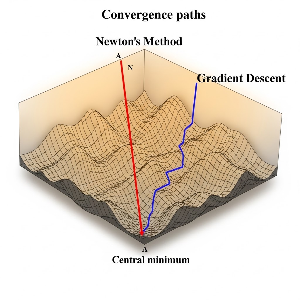
Steepest Descent
\[ x_{k+1}=x_k-s_k\nabla F(x_k), \] where \(s_k\) is step size (learning rate).
Steepest descent follows the negative gradient direction. Step size is critical: too large overshoots; too small converges slowly.
Newton’s Method
\[ x_{k+1}=x_k-H(x_k)^{-1}\nabla F(x_k). \]
Compared with steepest descent, Newton uses local curvature to adapt direction and scale.
Convexity
Convex set
A set \(C\) is convex if \[ x,y\in C,\ \forall\theta\in[0,1]\Longrightarrow\theta x+(1-\theta)y\in C. \]
Convex function
A function \(f\) is convex if \[ f(\theta x+(1-\theta)y)\le \theta f(x)+(1-\theta)f(y),\quad x,y\in\mathrm{dom}(f),\ \theta\in[0,1]. \]
From calculus, in 1D, \(f''(x)\ge 0\) implies convexity. In optimization, convexity gives the key guarantee: every local minimum is also a global minimum.
Takeaway. Hessian and Jacobian connect multivariable calculus to practical optimization: gradient methods use first-order information, Newton uses second-order curvature, and convexity tells us when local optimization gives globally correct answers.