MIT 18.065: Lecture 22 - Gradient Descent
Gradient descent is a fundamental algorithm for minimizing a function, but its behavior is controlled by curvature, step size, and condition number.
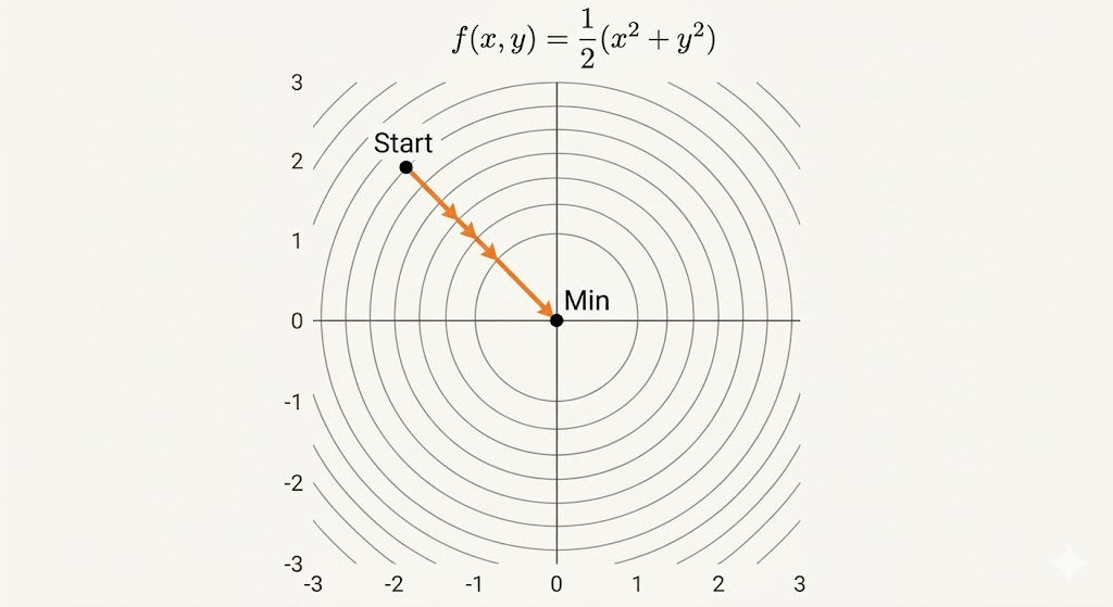
A Quadratic Matrix
\[ f(v)=\frac{1}{2}v^\top S v=\frac{1}{2}(x^2+b y^2), \qquad S=\begin{bmatrix}1&0\\0&b\end{bmatrix}, \qquad v=\begin{bmatrix}x\\y\end{bmatrix}. \]
This is the standard bowl model for analyzing gradient methods.
Gradient
For a linear function \[ f(x,y)=2x+5y, \] its gradient is \[ \nabla f=\begin{bmatrix}2\\5\end{bmatrix}, \] and the Hessian is zero: \[ H=\nabla^2 f=\begin{bmatrix}0&0\\0&0\end{bmatrix}. \]
So linear functions have constant slope and no curvature.
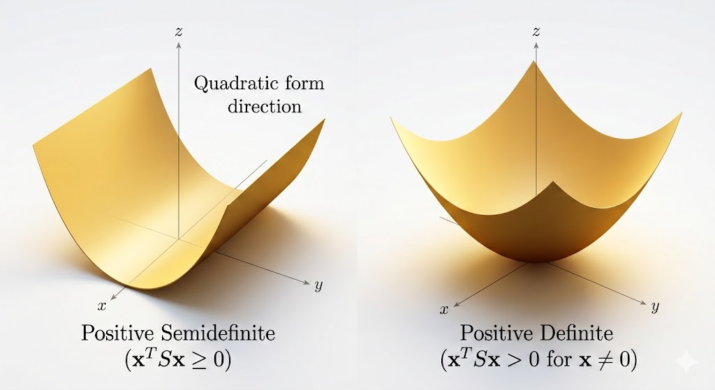
Hessian and Convexity
Definitions
- Convex: Hessian is positive semidefinite (PSD).
- Strictly convex: Hessian is positive definite (PD).
In eigenvalue language:
- PSD means \(\lambda_i\ge 0\) for all \(i\) (flat directions are allowed).
- PD means \(\lambda_i>0\) for all \(i\) (curvature in every direction).
Consequences:
- PSD convex objective: global minima exist, but may not be unique.
- PD objective: global minimum is unique.
Example
\[ f(x)=\frac{1}{2}x^\top Sx-a^\top x-b. \]
Then
- \(\nabla f = Sx-a\)
- \(H=\nabla^2 f=S\)
The minimizer solves \[ Sx-a=0 \quad\Rightarrow\quad x^*=S^{-1}a, \] assuming \(S\) is invertible.
A Remarkable Convex Function
\[ f(X)=-\log\det(X),\qquad X\in\mathbb{S}_{++}^n. \]
A key identity from matrix calculus is \[ \frac{\partial \log\det X}{\partial X_{ij}}=(X^{-1})_{ji}, \] so \[ \nabla_X\big(-\log\det X\big)=-X^{-\top}. \]
This function appears throughout optimization (barrier methods, covariance estimation, SDP-type models).
Gradient Descent
\[ x_{k+1}=x_k-s_k\nabla f(x_k), \] where \(s_k\) is the step size (learning rate).
Line Search Strategies
Exact Line Search
Choose \[ s_k=\arg\min_{s>0} f\big(x_k-s\nabla f(x_k)\big), \] so each step is optimal along the current descent line.
Backtracking Line Search
Start from a candidate step (often large), then shrink it until sufficient decrease is satisfied.
This is usually cheaper and more practical than exact line search.
Condition Number and Reduction
For quadratic objectives, convergence speed is governed by the condition number \[ \kappa=\frac{M}{m}, \] where \(M\) and \(m\) are largest/smallest Hessian eigenvalues.
- Well-conditioned (\(\kappa\approx 1\)): level sets are close to circles, gradients point toward the minimizer, and convergence is fast.
- Ill-conditioned (\(\kappa\gg 1\)): level sets are elongated, iterates zigzag across valleys, and convergence is slow.
A classical reduction factor with exact line search behaves like \[ \rho\approx\frac{\kappa-1}{\kappa+1}, \] so larger \(\kappa\) means slower progress per step.
Takeaway. Gradient descent performance is not just about choosing a learning rate. The geometry of the objective (through Hessian eigenvalues and condition number) is the central factor determining whether optimization is smooth or painfully slow.