MIT 18.065: Lecture 26 - Structure of Neural Nets for Deep Learning

Neural-network terminology, layer dimensions, weights and biases, function composition, and the geometric view of ReLU networks as continuous piecewise linear maps built by repeated folding.

This lecture shifts from optimization to the structure of neural networks themselves. The main message is geometric: a deep ReLU network is a composition of affine maps and nonlinear activations, and that composition produces a continuous piecewise linear function.

Terms

Training Data

Suppose the training set contains feature vectors

\[ x^{(1)}, x^{(2)}, \dots, x^{(N)} \in \mathbb{R}^m. \]

Each sample is an \(m\)-dimensional vector:

\[ x = \begin{bmatrix} x_1 \\ \vdots \\ x_m \end{bmatrix}. \]

Classification

For binary classification, the sign of the output determines the predicted class:

• if the label is \(+1\), we want \(F(x) > 0\)
• if the label is \(-1\), we want \(F(x) < 0\)

Activation Function

The standard ReLU activation is

\[ \operatorname{ReLU}(x) = \max(0,x). \]

ReLU is nonlinear, and that nonlinearity is what allows the network to represent nonlinear behavior.

Hidden Layer

A hidden layer is an intermediate layer between the input and the output.

• it receives the output of the previous layer
• it applies a new affine map plus activation
• it is called “hidden” because it is not directly the input data or the final prediction

Weights

The weights are the entries of the matrix \(A_\ell\) in layer \(\ell\).

They determine how strongly each coordinate from the previous layer influences each neuron in the next layer.

Bias

The bias vector \(b_\ell\) shifts the affine map before activation.

Without bias, every affine map would be forced to pass through the origin, which would make the network less flexible.

Output Layer

The output layer is the final layer that produces the prediction:

• for binary classification, it may output one score whose sign determines the class
• for multi-class classification, it may output several scores, one for each class
• depending on the task, the final activation may be identity, sigmoid, or softmax

Epochs

An epoch is one full pass through the training data.

With mini-batch SGD:

1. each step processes one mini-batch and updates the parameters once
2. one epoch is completed when the processed mini-batches together cover the full training set
3. before the next epoch, the data are usually shuffled and visited again

Structure of a Network

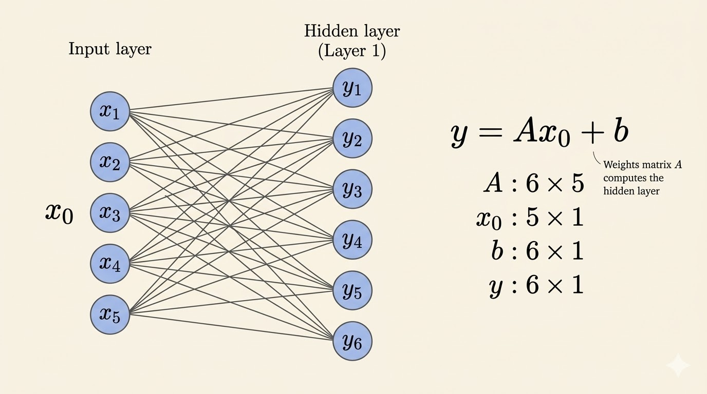
To keep the notation simple, start with the smallest nontrivial example: one input layer, one hidden layer, and one output layer.

Assume:

• the input layer has dimension \(n\)
• the hidden layer has dimension \(m\)
• the output layer comes after that hidden layer

Then the map from input to hidden layer uses:

• the weight matrix is \(A_1 \in \mathbb{R}^{m \times n}\)
• the bias vector is \(b_1 \in \mathbb{R}^m\)

The first affine map is

\[ y_1 = A_1 x_0 + b_1, \]

where \(x_0\) is the input vector.

After the activation, the hidden representation becomes

\[ x_1 = \sigma(y_1). \]

This is only a very simple example meant to show the dimensions and notation. A deep network just repeats the same pattern across many hidden layers.

So each layer does two things:

1. an affine transformation \(Ax+b\)
2. an elementwise nonlinear activation

Weight, Bias, and Activation

• \(A_\ell\): mixes coordinates from the previous layer
• \(b_\ell\): shifts the affine map
• \(\sigma\): bends the geometry by applying a nonlinear rule coordinate-wise

This pattern repeats layer by layer.

Composition of Functions

A deep network is a composition of functions:

\[ F(x) = F_3(F_2(F_1(x))). \]

For example:

• \(F_1(x) = \operatorname{ReLU}(A_1x+b_1)\)
• \(F_2(x) = \operatorname{ReLU}(A_2x+b_2)\)
• \(F_3(x) = \operatorname{sigmoid}(A_3x+b_3)\)

So deep learning is literally deep function composition.

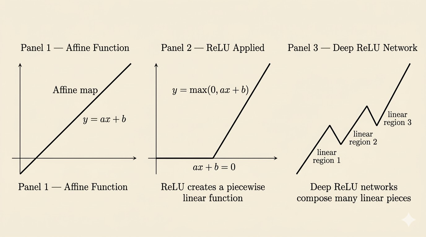
Continuous Piecewise Linear Functions

A continuous piecewise linear function is built from multiple linear pieces that join continuously.

• piecewise linear: the input space is divided into regions, and within each region the function is affine
• continuous: neighboring regions meet without gaps or jumps

For networks built from affine maps and ReLU activations, this is exactly what happens: the network is globally nonlinear, but locally affine on each region.

ReLU as a Folding Operation

ReLU networks can be viewed geometrically as repeatedly folding space.

Each layer first applies an affine transformation, then ReLU introduces a boundary where the slope changes. In higher dimensions, that boundary is a hyperplane. Each new hyperplane can split existing regions into smaller affine pieces.

To count the maximum number of regions cut by \(N\) hyperplanes in \(\mathbb{R}^m\), let

\[ R(N,m) \]

denote that maximum. Then the standard recursion is

\[ R(N,m) = R(N-1,m) + R(N-1,m-1). \]

Interpretation:

• \(R(N-1,m)\): the regions that already existed
• \(R(N-1,m-1)\): the new regions created when the new hyperplane cuts across old ones

Expanding the recursion gives the closed form

\[ R(N,m) = \sum_{k=0}^{m} \binom{N}{k}. \]

This is the maximum number of regions formed by \(N\) hyperplanes in \(m\) dimensions.

Example: Two-Dimensional Case

For \(m=2\),

\[ R(N,2) = \binom{N}{0} + \binom{N}{1} + \binom{N}{2}. \]

With \(N=3\),

\[ R(3,2) = 1 + 3 + 3 = 7. \]

So three folds in the plane can create at most seven regions.

For neural networks, the exact region count across many layers is more complicated than a single hyperplane arrangement, but the intuition is the same: more neurons and more layers create more affine pieces, which increases expressive power.

Takeaways

• A neural network layer applies an affine map followed by a nonlinear activation.
• ReLU is the key nonlinearity in this lecture, and it preserves continuity while creating piecewise linear structure.
• Deep networks are compositions of simpler functions.
• ReLU networks are globally nonlinear but locally affine on each region.
• Geometrically, deeper networks can be understood as repeatedly folding space into many linear pieces.

Source: MIT 18.065 Matrix Methods in Data Analysis, Signal Processing, and Machine Learning, Lecture 26.