Gilbert Strang’s Calculus: Linear Approximation and Newton’s Method
This lecture shows how the derivative gives the best local linear model of a function. That same tangent-line idea becomes Newton’s method when the goal is not to approximate a function value, but to find a root.
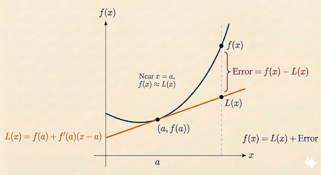
Linear Approximation
Start from the derivative at a point \(a\):
\[ f'(a) = \lim_{x \to a}\frac{f(x)-f(a)}{x-a}. \]
When \(x\) is close to \(a\), we treat the difference quotient as approximately equal to the derivative:
\[ f'(a) \approx \frac{f(x)-f(a)}{x-a}. \]
Rearranging gives the linear approximation formula
\[ f(x) \approx f(a) + f'(a)(x-a). \]
So near \(x=a\), the function is approximated by its tangent line.
Newton’s Method
Now suppose we want to solve
\[ F(x)=0. \]
Linearize \(F\) near a current guess \(a\):
\[ F(x) \approx F(a) + F'(a)(x-a). \]
At a root, the left-hand side should be \(0\), so set the approximation equal to zero:
\[ 0 \approx F(a) + F'(a)(x-a). \]
Solve for the improved estimate:
\[ x \approx a - \frac{F(a)}{F'(a)}. \]
This becomes the Newton iteration
\[ x_{n+1} = x_n - \frac{F(x_n)}{F'(x_n)}. \]
Newton’s method is therefore just tangent-line approximation applied repeatedly to the equation \(F(x)=0\).
Example 1: Approximating \(\sqrt{9.06}\)
Take
\[ f(x) = \sqrt{x}. \]
Choose the nearby point \(a=9\), where
\[ f(9)=3, \qquad f'(x)=\frac{1}{2\sqrt{x}}, \qquad f'(9)=\frac{1}{6}. \]
Then
\[ \sqrt{9.06} \approx 3 + \frac{1}{6}(9.06-9) = 3 + \frac{0.06}{6} = 3.01. \]
The local linear model already gives a very accurate approximation.
Newton Version of the Same Problem
To compute \(\sqrt{9.06}\) with Newton’s method, define
\[ F(x)=x^2-9.06. \]
We want the root of \(F(x)=0\). Start with the guess \(a=3\). Then
\[ F(3)=9-9.06=-0.06, \qquad F'(x)=2x, \qquad F'(3)=6. \]
Newton’s update gives
\[ x_1 = 3 - \frac{-0.06}{6} = 3.01. \]
This matches the linear-approximation answer.
Error After One Step
The approximation \(3.01\) is already close:
\[ 3.01^2 = 9.0601. \]
So the residual error in the squared value is
\[ 9.0601 - 9.06 = 0.0001. \]
Example 2: Approximating \(e^{0.01}\)
Take
\[ f(x)=e^x. \]
Use the nearby point \(a=0\):
\[ f(0)=1, \qquad f'(0)=1. \]
The linear approximation becomes
\[ e^x \approx 1 + x. \]
So at \(x=0.01\),
\[ e^{0.01} \approx 1.01. \]
This is a clean example of what linear approximation really keeps: the constant term and the first-order slope.
Newton’s Method: Second Iteration and Error Reduction
Continue the square-root example with the improved guess
\[ a=3.01. \]
Then
\[ F(a)=3.01^2-9.06=0.0001, \]
and
\[ F'(a)=2(3.01)=6.02. \]
Apply Newton’s formula again:
\[ x_2 = 3.01 - \frac{0.0001}{6.02} \approx 3.0099834. \]
Now the residual is dramatically smaller:
\[ F(x_2) \approx 2.76 \times 10^{-10}. \]
That is the striking feature of Newton’s method near a good starting point: the error can drop extremely fast, often with roughly quadratic convergence.
Takeaways
- Linear approximation says a smooth function looks like its tangent line locally.
- Newton’s method uses that same tangent line to jump toward a root.
- For \(\sqrt{9.06}\), both approaches produce the first estimate \(3.01\).
- Repeating Newton’s update gives much faster error reduction than a single linear approximation.
Source: Gilbert Strang’s Calculus lecture on linear approximation and Newton’s method.