MIT 18.065: Lecture 25 - Stochastic Gradient Descent

Finite-sum objectives, why SGD is cheaper than full gradient descent, why it fluctuates near the optimum, and how unbiased stochastic gradients, reshuffling, and mini-batches make large-scale learning practical.

Many optimization problems in machine learning have the same structure: the objective is an average of per-sample losses. This lecture explains why that structure leads naturally to stochastic gradient descent, and why the noise in SGD is both its strength and its limitation.

Finite-Sum Problems

A large class of models can be written as

\[ f(x)=\frac{1}{n}\sum_{i=1}^n f_i(x). \]

Examples:

Least Squares

\[ \frac{1}{n}\|Ax-b\|^2 = \frac{1}{n}\sum_{i=1}^n (a_i^\top x-b_i)^2 = \frac{1}{n}\sum_{i=1}^n f_i(x). \]

Lasso

\[ \frac{1}{n}\|Ax-b\|^2+\lambda \|x\|_1 = \frac{1}{n}\sum_{i=1}^n (a_i^\top x-b_i)^2 + \lambda \sum_j |x_j|. \]

Support Vector Machine

\[ \frac{1}{2}\|x\|_2^2 + \frac{C}{n}\sum_{i=1}^n \max\bigl(0,1-y_i(x^\top a_i+b)\bigr). \]

Deep Neural Networks

\[ \frac{1}{n}\sum_{i=1}^n \text{loss}\bigl(y_i,\mathcal{DNN}(x;a_i)\bigr) = \frac{1}{n}\sum_{i=1}^n f_i(x). \]

This finite-sum form is the reason SGD exists as a specialized optimization method.

Why SGD?

Full gradient descent uses

\[ x_{k+1}=x_k-\eta_k \nabla f(x_k) = x_k-\eta_k \frac{1}{n}\sum_{i=1}^n \nabla f_i(x_k). \]

The drawback is cost: when \(n\) is huge, computing the whole gradient every step is too expensive.

SGD replaces the full average with one randomly selected sample index \(i(k)\):

\[ x_{k+1}=x_k-\eta_k \nabla f_{i(k)}(x_k). \]

Each update is roughly \(n\) times cheaper, which is why SGD scales to massive datasets.

One-sample updates make each iteration much cheaper

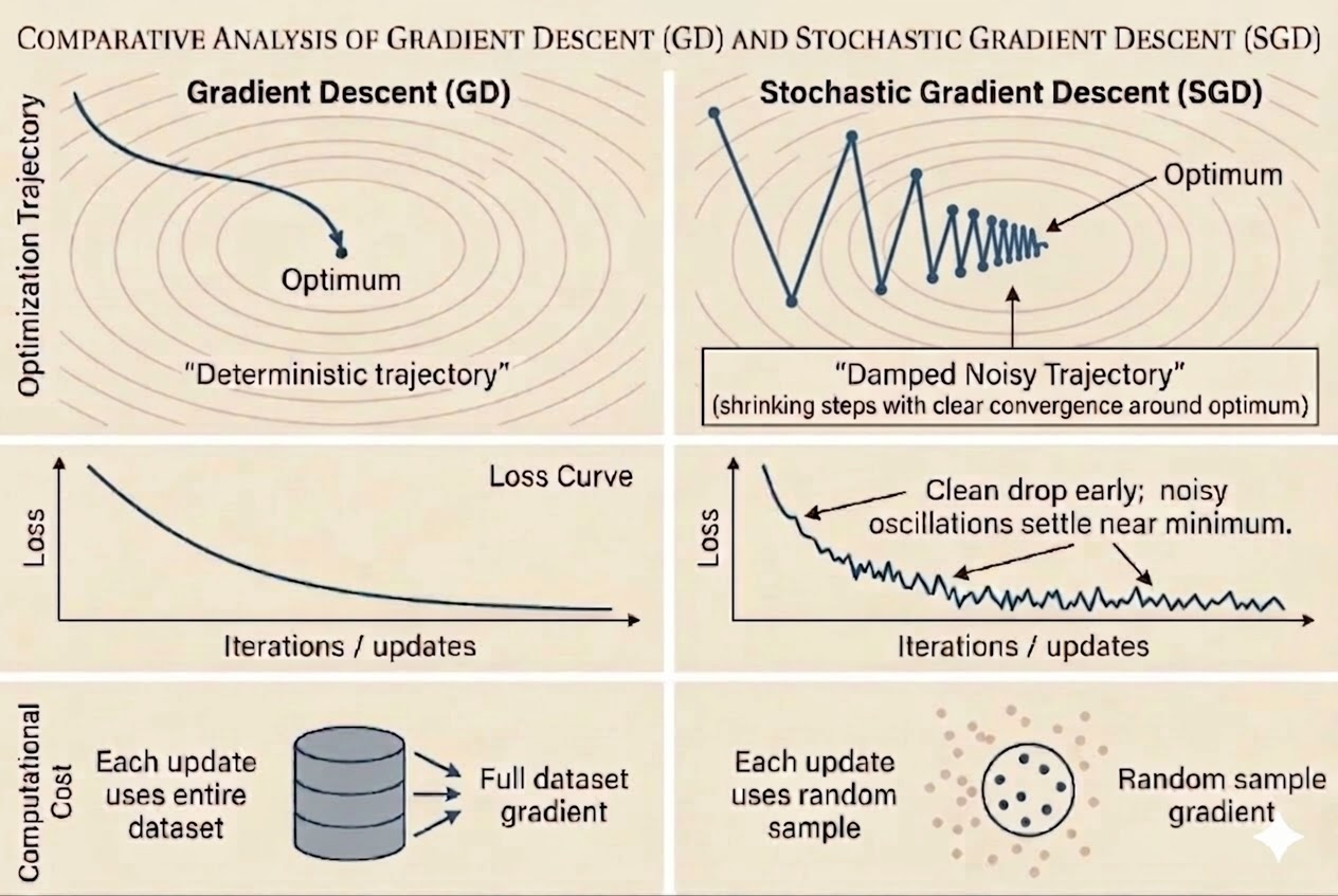
Why SGD Fluctuates

A common empirical pattern is:

• early iterations drop the loss quickly
• near the optimum, the iterates fluctuate instead of settling smoothly

SGD often oscillates near the optimum

This is not a bug. It is the direct consequence of using noisy per-sample gradients.

Geometric Intuition

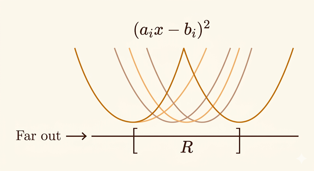
Consider a 1D least-squares objective where each sample contributes

\[ f_i(x)=(a_i x-b_i)^2. \]

Each \(f_i\) is its own parabola with its own minimizer

\[ x_i^*=\frac{b_i}{a_i}. \]

Let

\[ R=[\min_i x_i^*,\max_i x_i^*]. \]

Then the global optimum of the whole dataset lies somewhere inside this region.

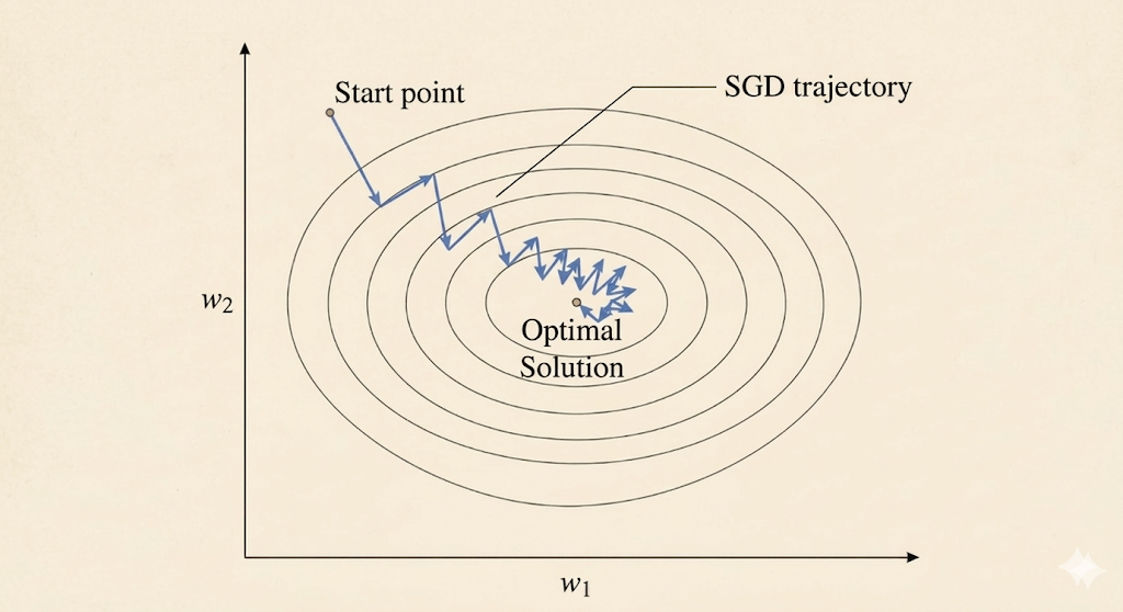
Two phases explain the SGD dynamics:

1. Far outside \(R\), all sample gradients roughly point in the same direction, so SGD moves consistently toward the solution region.
2. Inside \(R\), different samples pull in different directions, creating a tug-of-war that makes the iterates bounce around.

Individual sample minima create a tug-of-war near the optimum

This is why SGD needs either a decaying learning rate or averaging if we want the fluctuations to shrink.

The Key Idea: Unbiased Gradient Estimates

SGD works because its noisy gradient is unbiased:

\[ \mathbb{E}[g(x)] = \nabla f(x). \]

Here:

• \(\nabla f(x)\) is the true full-dataset gradient
• \(g(x)\) is the stochastic gradient from one random sample

A single stochastic step may point in a bad direction, but on average these steps line up with the true descent direction.

That is the central tradeoff:

• exact gradient: expensive and stable
• stochastic gradient: cheap and noisy

Two Sampling Variants

With Replacement

At each step, pick an index uniformly from \(\{1,\dots,n\}\) independently of previous picks.

• easiest to analyze mathematically
• standard form in convergence proofs
• can revisit some samples many times before seeing others

Without Replacement

Shuffle the dataset once per epoch and then visit each sample exactly once.

• standard in practical machine learning code
• usually converges faster in practice
• harder to analyze theoretically

This is the difference between textbook SGD and the reshuffling used in most libraries.

Mini-Batch SGD

Mini-batch SGD averages a small subset \(J_k\) of samples:

\[ x_{k+1} = x_k-\frac{\eta_k}{|J_k|}\sum_{j\in J_k}\nabla f_j(x_k). \]

It sits between:

• batch gradient descent: use all samples
• SGD: use one sample

Why mini-batches matter:

• GPUs are efficient on matrix-matrix operations, so processing 32 or 64 samples together is often almost as cheap as processing one
• distributed training reduces communication overhead by synchronizing less often
• a little noise can help optimization and generalization

Very large mini-batches are not always favorable for deep learning, because they reduce gradient noise and can hurt the final generalization behavior.

Takeaways

• Many ML objectives are finite sums, which makes SGD a natural algorithmic match.
• SGD is cheap because it replaces the full gradient by one sample or a small batch.
• Near the optimum, sample gradients conflict, so fluctuations are expected.
• The reason SGD still works is unbiasedness: the noisy gradient points in the correct direction on average.
• In practice, shuffled passes and mini-batches are the default compromise between theory and hardware efficiency.

Source: MIT 18.065 Matrix Methods in Data Analysis, Signal Processing, and Machine Learning, Lecture 25.