MIT 6.041 Probability: Probability Models and Axioms

Sample spaces, discrete and continuous probability models, probability axioms, uniform laws, and counting examples from the opening lecture of MIT 6.041.

Sample Space \(\Omega\)

The sample space is the set of all possible outcomes of an experiment.

Two key properties:

• outcomes should be mutually exclusive
• outcomes should be collectively exhaustive

Examples:

• flipping a coin: {H, T}
• rolling a 4-sided die: {1,2,3,4}

Discrete Example

Consider rolling a 4-sided die twice.

Outcome Table

1st \ 2nd	1	2	3	4
1	(1,1)	(1,2)	(1,3)	(1,4)
2	(2,1)	(2,2)	(2,3)	(2,4)
3	(3,1)	(3,2)	(3,3)	(3,4)
4	(4,1)	(4,2)	(4,3)	(4,4)

Sequential Description

graph LR
    Start((Start)) --> A1((1))
    Start --> A2((2))
    Start --> A3((3))
    Start --> A4((4))

    A1 --> A11["(1,1)"]
    A1 --> A12["(1,2)"]
    A1 --> A13["(1,3)"]
    A1 --> A14["(1,4)"]

    A2 --> A21["(2,1)"]
    A2 --> A22["(2,2)"]
    A2 --> A23["(2,3)"]
    A2 --> A24["(2,4)"]

    A3 --> More1["..."]
    A4 --> More2["..."]

The table and the tree describe the same sample space. One is geometric, the other is sequential.

Continuous Example

For a continuous model,

\[ \Omega = \{(x,y)\mid 0 \le x,y \le 1\}. \]

The probability of any exact point is 0, because a point has no area.

So in continuous probability, we do not assign probability to single points. We assign probability to regions.

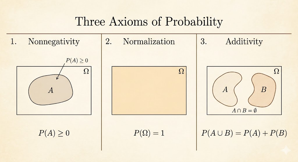
Axioms

The core axioms are:

• nonnegativity: \(P(A) \ge 0\)
• normalization: \(P(\Omega) = 1\)
• additivity: if \(A \cap B = \emptyset\), then \(P(A \cup B) = P(A) + P(B)\)

For infinite sample spaces, this extends to countable additivity:

If \(A_1, A_2, \dots\) are disjoint, then

\[ P(A_1 \cup A_2 \cup \cdots) = P(A_1) + P(A_2) + \cdots \]

From the axioms we can derive useful facts. For example, probability is always at most 1.

Since

\[ P(\Omega) = P(A) + P(A^c) = 1 \]

and

\[ P(A^c) \ge 0, \]

it follows that

\[ P(A) \le 1. \]

Exercise

Use the 4 x 4 dice example, where each outcome has probability 1/16.

Y \ X	1	2	3	4
4	(1,4)	(2,4)	(3,4)	(4,4)
3	(1,3)	(2,3)	(3,3)	(4,3)
2	(1,2)	(2,2)	(3,2)	(4,2)
1	(1,1)	(2,1)	(3,1)	(4,1)

Examples:

• \(P\big((X,Y)\in\{(1,1),(1,2)\}\big)=\frac{2}{16}=\frac{1}{8}\)
• \(P(X=1)=\frac{4}{16}=\frac{1}{4}\)
• \(P(X+Y \text{ is odd})=\frac{8}{16}=\frac{1}{2}\)
• \(P(\min(X,Y)=2)=\frac{5}{16}\)

Discrete Uniform Law

If all outcomes are equally likely, then

\[ P(A)=\frac{\text{number of elements of }A}{\text{total number of sample points}}. \]

So computing probability becomes a counting problem.

Continuous Uniform Law

In a continuous uniform model, probability is proportional to length, area, or volume.

That is why:

• a single point has probability 0
• intervals or regions can have positive probability

For continuous models, probability is geometric rather than combinatorial.

Takeaways

• the sample space is the formal description of all possible outcomes
• discrete and continuous models behave differently: counting versus geometry
• the probability axioms are simple, but they generate the whole framework
• uniform probability reduces many problems to either counting or area