Lecture 27: Back Propagation and Partial Gradients

Backpropagation as reverse-mode differentiation: a chain-rule view of neural networks, a worked partial-gradient example, and why the backward order is far cheaper than naive Jacobian multiplication.

This lecture explains backpropagation as the chain rule applied efficiently to a nested function. The point is not just how to differentiate a deep network, but why the backward order is computationally the right one.

Structure of Deep Learning

A deep network is a composition of functions:

\[ F(x)=F_3(F_2(F_1(x))). \]

Every layer takes the output of the previous layer and applies another transformation. Backpropagation computes how the final output changes with respect to each earlier variable or parameter.

Example Function

Use

\[ F(x,y)=x^3(x+3y). \]

Introduce intermediate variables:

\[ C=x^3,\qquad S=x+3y,\qquad F=C\cdot S. \]

This turns one expression into a short computational graph.

A simple computational graph for the chain-rule example

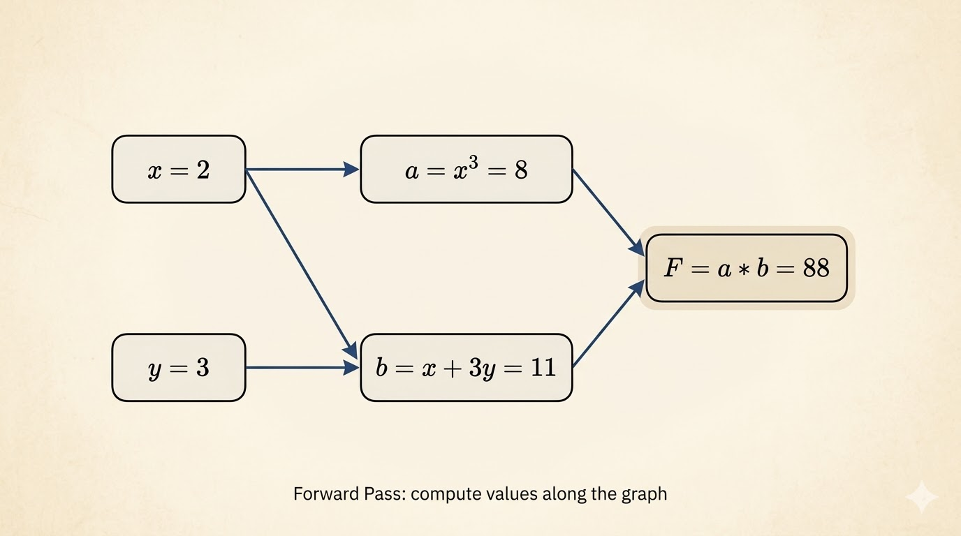
Forward Propagation

Take the concrete point

\[ x=2,\qquad y=3. \]

Then the forward pass is

\[ C=x^3=8,\qquad S=x+3y=11,\qquad F=C\cdot S=88. \]

The forward sweep computes values once and stores them for later reuse.

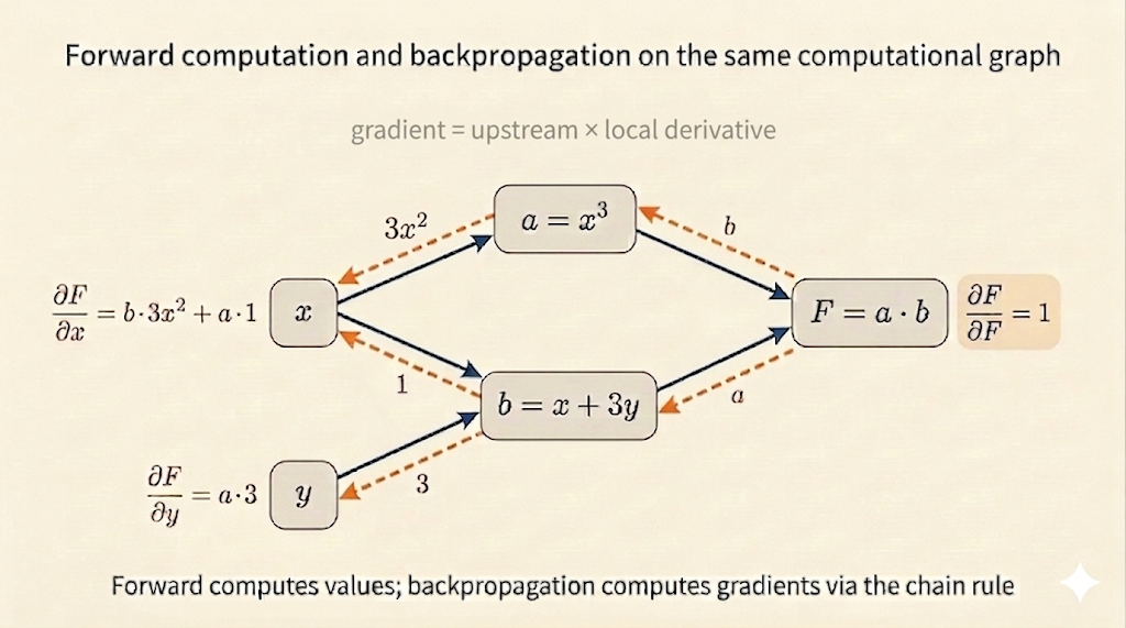
Local Derivatives

Backpropagation needs only local derivatives at each node:

\[ \frac{\partial C}{\partial x}=3x^2,\qquad \frac{\partial S}{\partial x}=1,\qquad \frac{\partial S}{\partial y}=3. \]

At \(x=2\),

\[ \frac{\partial C}{\partial x}=3(2)^2=12. \]

For the product node,

\[ \frac{\partial F}{\partial S}=C,\qquad \frac{\partial F}{\partial C}=S. \]

At the forward-pass values,

\[ \frac{\partial F}{\partial S}=8,\qquad \frac{\partial F}{\partial C}=11. \]

Back Propagation

Now sweep backward from the output:

\[ \frac{\partial F}{\partial F}=1. \]

Then propagate through the graph:

\[ \frac{\partial F}{\partial S}=C=8,\qquad \frac{\partial F}{\partial C}=S=11. \]

Finally combine these with the earlier local derivatives:

\[ \frac{\partial F}{\partial x} = \frac{\partial F}{\partial S}\frac{\partial S}{\partial x} + \frac{\partial F}{\partial C}\frac{\partial C}{\partial x} =8\cdot 1+11\cdot 12=140, \]

and

\[ \frac{\partial F}{\partial y} = \frac{\partial F}{\partial S}\frac{\partial S}{\partial y} =8\cdot 3=24. \]

This is the core logic of backpropagation: the gradient at one node is the downstream gradient multiplied by the local derivative.

Famous Derivatives and Automatic Differentiation

Backpropagation reuses a small library of basic derivatives:

• \(x^n \mapsto nx^{n-1}\)
• \(\sin x \mapsto \cos x\)
• \(\cos x \mapsto -\sin x\)
• \(e^x \mapsto e^x\)
• \(\log x \mapsto \frac{1}{x}\)

Automatic differentiation systems assemble these local rules into a full reverse sweep over the computational graph.

Chain Rule Through a Network

For a deep network, the gradient of the loss with respect to an earlier parameter is a chain of derivatives:

\[ \frac{\partial \text{Loss}}{\partial w_i} = \frac{\partial \text{Loss}}{\partial \text{layer}_n} \cdot \frac{\partial \text{layer}_n}{\partial \text{layer}_{n-1}} \cdots \frac{\partial \text{layer}_{i+1}}{\partial w_i}. \]

So each parameter’s influence is filtered through every layer that comes after it.

This explains two practical facts:

• earlier layers depend on feedback from downstream layers
• if those downstream derivatives are tiny, the gradient signal can shrink, producing vanishing gradients

Backward gradient flow through the chain of layers

Why Reverse-Mode Differentiation Is Efficient

The mathematics behind backpropagation is the associativity of matrix multiplication:

\[ A(BC)=(AB)C. \]

The final answer is the same either way, but the cost can be radically different.

Suppose

\[ A:1\times 100,\qquad B:100\times 100,\qquad C:100\times 1000. \]

Then:

• left-to-right style computes \[ BC:\ 100\cdot100\cdot1000=10,\!000,\!000 \] operations first, producing a large intermediate matrix
• right-to-left style computes \[ AB:\ 1\cdot100\cdot100=10,\!000 \] operations first, producing only a row vector

The second step costs the same in both cases:

\[ 1\cdot100\cdot1000=100,\!000. \]

So the totals are:

Order	Total Multiplications
\(A(BC)\)	\(10,\!100,\!000\)
\((AB)C\)	\(110,\!000\)

This is the key computational insight:

• forward-mode can force large matrix-matrix intermediates
• reverse-mode starts from the scalar loss and keeps intermediate objects small
• backpropagation therefore gets all partial gradients at much lower cost

Takeaways

• A deep network is a chain of functions, so its gradients come from repeated chain-rule application.
• Forward propagation computes and stores intermediate values.
• Backpropagation reuses those intermediates and multiplies local derivatives backward.
• The reverse order is not just mathematically correct; it is computationally much cheaper.

Source: MIT 18.065 Lecture 27 on back propagation and partial gradients.