Lecture 30: Completing a Rank-1 Matrix, Circulants
This lecture combines two ideas that look separate at first:
- how to complete a rank-1 matrix from a small number of entries
- why circulant matrices are really convolution operators in disguise
Completing a Rank-1 Matrix
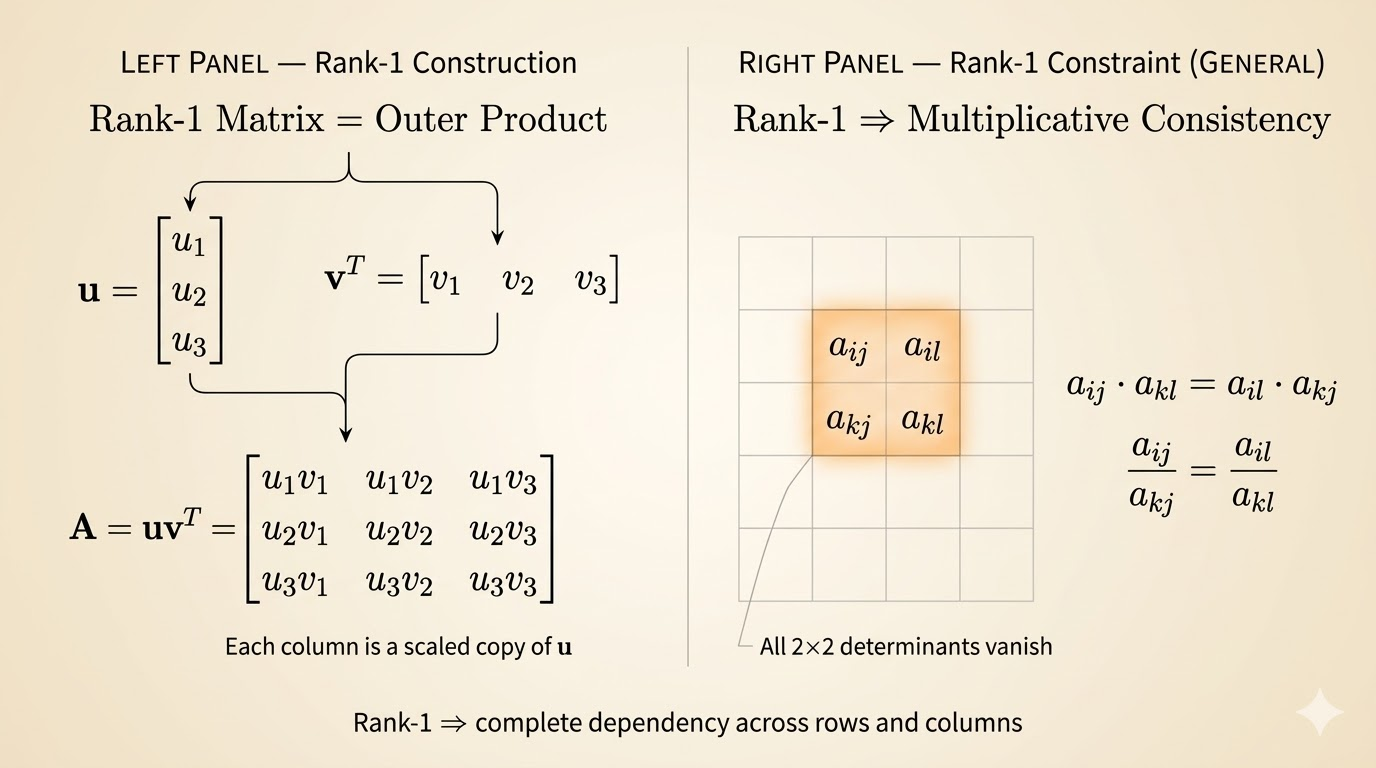
A rank-1 matrix has the form
\[ A = uv^\top \]
where both \(u\) and \(v\) are column vectors. Entrywise,
\[ a_{ij} = u_i v_j \]
So once the row factors and column factors are fixed, the whole matrix is determined.
For an \(m \times n\) rank-1 matrix, we need only
\[ m+n-1 \]
entries to determine the rest, provided those entries are placed in the right pattern and are nonzero.
For example, a \(3 \times 3\) rank-1 matrix needs only
\[ 3+3-1 = 5 \]
entries.
Why Some Choices Fail
The count \(m+n-1\) is necessary, but it is not sufficient by itself. The positions of the known entries matter.
Algebraic View: Every \(2 \times 2\) Minor Must Vanish
In a rank-1 matrix, every \(2 \times 2\) submatrix must have determinant zero. So if we prescribe four arbitrary nonzero values in a full \(2 \times 2\) block, they usually violate
\[ a_{11}a_{22} = a_{12}a_{21} \]
and completion fails immediately.
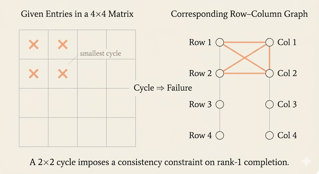
Graph View: Cycles Mean Failure
Professor Strang turns the same condition into a bipartite graph:
- left nodes are rows
- right nodes are columns
- each known entry is an edge between a row and a column
The rule is:
Cycle = failure.
If the known entries form a cycle, then they impose one redundant constraint too many, which usually creates a contradiction. The successful pattern is a spanning tree on the row-column bipartite graph.
Long Cycles Also Fail
The obstruction is not only a \(2 \times 2\) block. A longer cycle also causes failure.
For example, a length-6 cycle inside a local \(3 \times 3\) region prescribes too many entries for a rank-1 structure. A \(3 \times 3\) rank-1 block only needs
\[ 3+3-1 = 5 \]
entries, so six arbitrary nonzero entries typically overconstrain it.
The graph interpretation is the clean summary:
- no cycle: completion is possible
- any cycle: completion fails
Circulant Matrices
A circulant matrix is a square matrix where each row is a cyclic shift of the previous row. For example,
\[ \begin{bmatrix} 2 & 1 & 0 & 5 \\ 5 & 2 & 1 & 0 \\ 0 & 5 & 2 & 1 \\ 1 & 0 & 5 & 2 \end{bmatrix} \]
can be built from the cyclic permutation matrix
\[ P = \begin{bmatrix} 0 & 1 & 0 & 0 \\ 0 & 0 & 1 & 0 \\ 0 & 0 & 0 & 1 \\ 1 & 0 & 0 & 0 \end{bmatrix} \]
together with the identity matrix
\[ I = \begin{bmatrix} 1 & 0 & 0 & 0 \\ 0 & 1 & 0 & 0 \\ 0 & 0 & 1 & 0 \\ 0 & 0 & 0 & 1 \end{bmatrix} \]
and its powers \(P^2, P^3\).
For instance,
\[ P^2 \begin{bmatrix} x_0 \\ x_1 \\ x_2 \\ x_3 \end{bmatrix} = \begin{bmatrix} x_2 \\ x_3 \\ x_0 \\ x_1 \end{bmatrix} \]
So powers of \(P\) just rotate the entries.
Every Circulant Matrix Is a Polynomial in \(P\)
Any \(n \times n\) circulant matrix can be written as
\[ C = c_0 I + c_1 P + c_2 P^2 + \cdots + c_{n-1}P^{n-1} \]
and similarly
\[ D = d_0 I + d_1 P + d_2 P^2 + \cdots + d_{n-1}P^{n-1} \]
Since
\[ P^n = I, \]
multiplying two such polynomials and reducing powers modulo \(n\) gives another circulant matrix. So:
- circulants are closed under multiplication
- matrix multiplication becomes polynomial multiplication modulo \(P^n=I\)
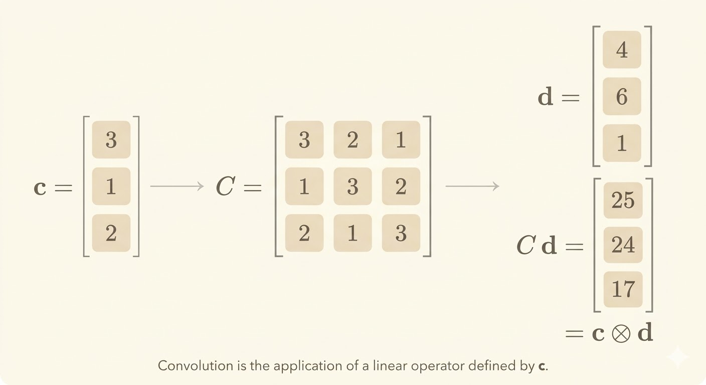
Matrix Multiplication = Circular Convolution
If
\[ C = \sum_i c_i P^i, \qquad D = \sum_j d_j P^j \]
then
\[ CD = \sum_k e_k P^k \]
where
\[ e_k = \sum_i c_i d_{k-i \;(\mathrm{mod}\; n)} \]
This is exactly circular convolution.
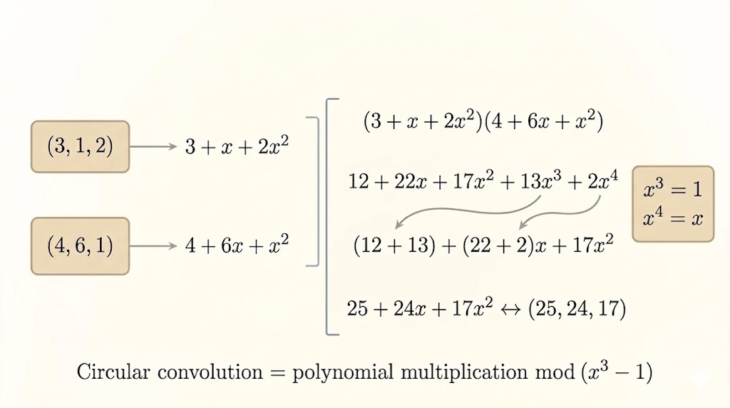
A Small Convolution Example
Take the vectors
\[ (3,1,2) \qquad \text{and} \qquad (4,6,1) \]
Interpret them as polynomials
\[ 3 + x + 2x^2 \qquad \text{and} \qquad 4 + 6x + x^2 \]
Their product is
\[ (3 + x + 2x^2)(4 + 6x + x^2) = 12 + 22x + 17x^2 + 8x^3 + 2x^4 \]
For length \(n=3\), circular convolution means working modulo
\[ x^3 - 1 \]
so
\[ x^3 = 1, \qquad x^4 = x \]
and therefore
\[ 12 + 22x + 17x^2 + 8x^3 + 2x^4 \equiv 20 + 24x + 17x^2 \]
Hence
\[ (3,1,2)\otimes(4,6,1) = (20,24,17) \]
Eigenvalues, Eigenvectors, and Fourier Modes
Because every circulant matrix is a polynomial in \(P\), circulant matrices share the eigenvectors of \(P\).
So we first solve
\[ Pv = \lambda v \]
with the condition
\[ P^n = I \]
which implies
\[ \lambda^n = 1 \]
Therefore the eigenvalues are the \(n\)th roots of unity:
\[ \lambda_k = \omega^k, \qquad \omega = e^{2\pi i/n}, \qquad k=0,\dots,n-1 \]
The corresponding eigenvectors are
\[ v_k = \begin{bmatrix} 1 \\ \omega^k \\ \omega^{2k} \\ \vdots \\ \omega^{(n-1)k} \end{bmatrix} \]
These are exactly the Fourier modes. That is why Fourier analysis diagonalizes circulant matrices.
Takeaways
- A rank-1 matrix is determined by \(m+n-1\) well-placed nonzero entries.
- The correct graph condition is tree vs cycle: any cycle creates failure.
- A circulant matrix is a polynomial in the shift matrix \(P\).
- Multiplying circulant matrices is the same as circular convolution.
- The eigenvectors of circulants are Fourier modes, coming from the roots of unity.