Gilbert Strang’s Calculus: Differential Equations of Growth
This lecture starts from the simplest growth law and then adds more realistic effects:
- pure exponential growth
- constant source terms
- logistic saturation
- predator-prey interaction
Basic Exponential Growth
The simplest growth model is
\[ \frac{dy}{dt} = cy \]
The growth rate is proportional to the current amount \(y\).
With initial value
\[ y(0) = y_0 \]
the solution is
\[ y(t) = y_0 e^{ct} \]
because
\[ \frac{d}{dt}(y_0 e^{ct}) = c y_0 e^{ct} = c y(t) \]
So:
- if \(c>0\), the quantity grows exponentially
- if \(c<0\), the quantity decays exponentially
Adding a Constant Source
Now include a source term:
\[ \frac{dy}{dt} = cy + s \]
This is a linear differential equation. Its solution can be written as
\[ y(t) = y_{\text{particular}}(t) + y_{\text{homogeneous}}(t) \]
Particular Solution
Try a constant solution. Then \(dy/dt = 0\), so
\[ 0 = cy + s \qquad \Rightarrow \qquad y = -\frac{s}{c} \]
So one particular solution is
\[ y_{\text{particular}} = -\frac{s}{c} \]
Homogeneous Solution
The associated homogeneous equation is
\[ \frac{dy}{dt} = cy \]
with solution
\[ Ae^{ct} \]
Therefore the full solution is
\[ y(t) = -\frac{s}{c} + Ae^{ct} \]
Using \(y(0)=y_0\) gives
\[ A = y_0 + \frac{s}{c} \]
so
\[ y(t) + \frac{s}{c} = \left(y_0 + \frac{s}{c}\right)e^{ct} \]
Logistic Population Growth
Pure exponential growth cannot continue forever. A common correction is the logistic equation:
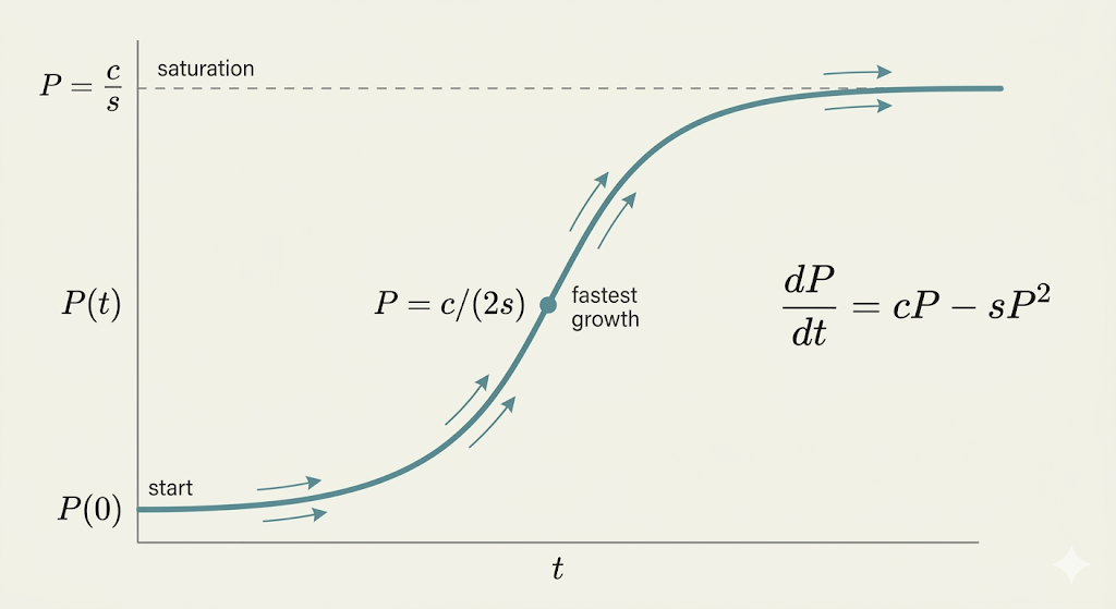
\[ \frac{dP}{dt} = cP - sP^2 \]
where
- \(c\) is the net growth rate
- \(s\) is the slowdown factor from competition
This can also be written as
\[ \frac{dP}{dt} = P(c-sP) \]
Early Stage
When \(P\) is small, the term \(sP^2\) is negligible, so the model behaves almost like
\[ \frac{dP}{dt} \approx cP \]
which is exponential growth.
Carrying Capacity
At equilibrium,
\[ \frac{dP}{dt}=0 \]
so
\[ cP - sP^2 = 0 \qquad \Rightarrow \qquad P = 0 \quad \text{or} \quad P = \frac{c}{s} \]
The positive steady state
\[ P = \frac{c}{s} \]
is the carrying capacity.
Inflection Point
The logistic curve grows fastest halfway to the carrying capacity:
\[ P = \frac{c}{2s} \]
That is where the graph changes from bending upward to bending downward.
Solving the Logistic Equation by Letting \(y = 1/P\)
Let
\[ y = \frac{1}{P} \]
Then by the chain rule,
\[ \frac{dy}{dt} = \frac{d}{dt}\left(\frac{1}{P}\right) = -\frac{1}{P^2}\frac{dP}{dt} \]
Substitute the logistic equation:
\[ \frac{dy}{dt} = -\frac{1}{P^2}(cP - sP^2) = s - c\frac{1}{P} = s - cy \]
So \(y\) satisfies the linear equation
\[ \frac{dy}{dt} = s - cy \]
whose solution is
\[ y(t) - \frac{s}{c} = \left(y(0) - \frac{s}{c}\right)e^{-ct} \]
Since \(y=1/P\), this becomes
\[ \frac{1}{P(t)} - \frac{s}{c} = \left(\frac{1}{P(0)} - \frac{s}{c}\right)e^{-ct} \]
This is the logistic solution in reciprocal form.
Predator-Prey Model
The lecture ends by moving from one population to two interacting populations.
Let
- \(u\) = predator population
- \(v\) = prey population
One standard model is
\[ \frac{du}{dt} = -cu + kuv \]
\[ \frac{dv}{dt} = Cv - suv \]
Interpretation:
- predators die out without prey because of the term \(-cu\)
- predators grow when predator-prey encounters happen, through \(kuv\)
- prey grows naturally through \(Cv\)
- prey decreases through predation, modeled by \(-suv\)
Unlike the logistic equation, which approaches a steady ceiling, the predator-prey system often produces oscillation:
- prey increases first
- predators then increase because food is abundant
- prey falls as predation rises
- predators then fall because food becomes scarce
and the cycle can repeat.
Takeaways
- \(\frac{dy}{dt}=cy\) gives pure exponential growth or decay.
- Adding a source term still leaves a linear ODE with a particular-plus-homogeneous structure.
- The logistic equation adds self-limiting competition and produces an S-curve.
- The substitution \(y=1/P\) turns the logistic equation into a linear equation.
- Coupling two growth equations leads naturally to predator-prey oscillations.