Lecture 31: Eigenvectors of Circulant Matrices, Fourier Matrix
A circulant matrix is built by shifting the first row cyclically:
\[ C = \begin{bmatrix} c_0 & c_1 & c_2 & \cdots & c_{N-1} \\ c_{N-1} & c_0 & c_1 & \cdots & c_{N-2} \\ c_{N-2} & c_{N-1} & c_0 & \cdots & c_{N-3} \\ \vdots & \vdots & \vdots & \ddots & \vdots \\ c_1 & c_2 & c_3 & \cdots & c_0 \end{bmatrix}. \]
The key idea of the lecture is that circulant matrices are governed by the cyclic shift matrix, and that shift matrix is diagonalized by Fourier vectors.
The Shift Matrix P
Let
\[ P = \begin{bmatrix} 0 & 1 & 0 & 0 \\ 0 & 0 & 1 & 0 \\ 0 & 0 & 0 & 1 \\ 1 & 0 & 0 & 0 \end{bmatrix}. \]
Multiplying by \(P\) shifts the entries of a vector upward by one position and wraps the first component to the bottom.
Every circulant matrix can be written as a polynomial in \(P\):
\[ C = c_0 I + c_1 P + c_2 P^2 + \cdots + c_{N-1} P^{N-1}. \]
So once the eigenvalues and eigenvectors of \(P\) are known, the same structure extends to every circulant matrix.
Eigenvalues of P
To find the eigenvalues, solve
\[ Px = \lambda x. \]
For the \(4 \times 4\) shift matrix, this is equivalent to solving
\[ \det(\lambda I - P) = 0. \]
The characteristic equation is
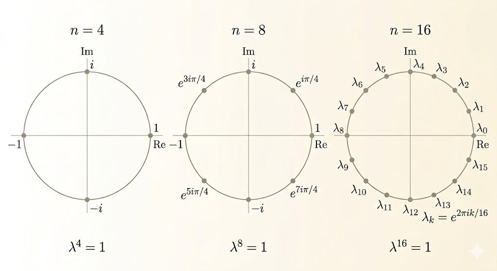
\[ \lambda^4 - 1 = 0, \]
so the eigenvalues are the fourth roots of unity:
- \(1\)
- \(i\)
- \(-1\)
- \(-i\)
Written in Euler form, these four values are
\[ e^{\pi i/2}=\cos(\pi/2)+i\sin(\pi/2)=i \]
\[ e^{\pi i}=\cos(\pi)+i\sin(\pi)=-1 \]
\[ e^{3\pi i/2}=\cos(3\pi/2)+i\sin(3\pi/2)=-i \]
\[ e^{2\pi i}=\cos(2\pi)+i\sin(2\pi)=1. \]
For the \(8 \times 8\) shift matrix, the characteristic equation becomes
\[ \lambda^8 = 1, \]
so the eigenvalues are the eight roots of unity:
- \(1\)
- \(e^{\pi i/4}\)
- \(i\)
- \(e^{3\pi i/4}\)
- \(-1\)
- \(e^{5\pi i/4}\)
- \(-i\)
- \(e^{7\pi i/4}\)
For an \(N \times N\) shift matrix, the same argument gives
\[ \lambda^N = 1, \]
so the eigenvalues are the \(N\)th roots of unity:
\[ 1,\; \omega,\; \omega^2,\; \dots,\; \omega^{N-1}, \qquad \omega = e^{2\pi i / N}. \]
This is the general solution: every eigenvalue of the shift matrix is a root of unity.
Why These Numbers Work
The proof is short:
\[ e^{2\pi i} = \cos(2\pi) + i\sin(2\pi) = 1. \]
So for any integer \(k\),
\[ \left(e^{2\pi i k / N}\right)^N = e^{2\pi i k} = 1. \]
That is exactly the condition \(\lambda^N = 1\).
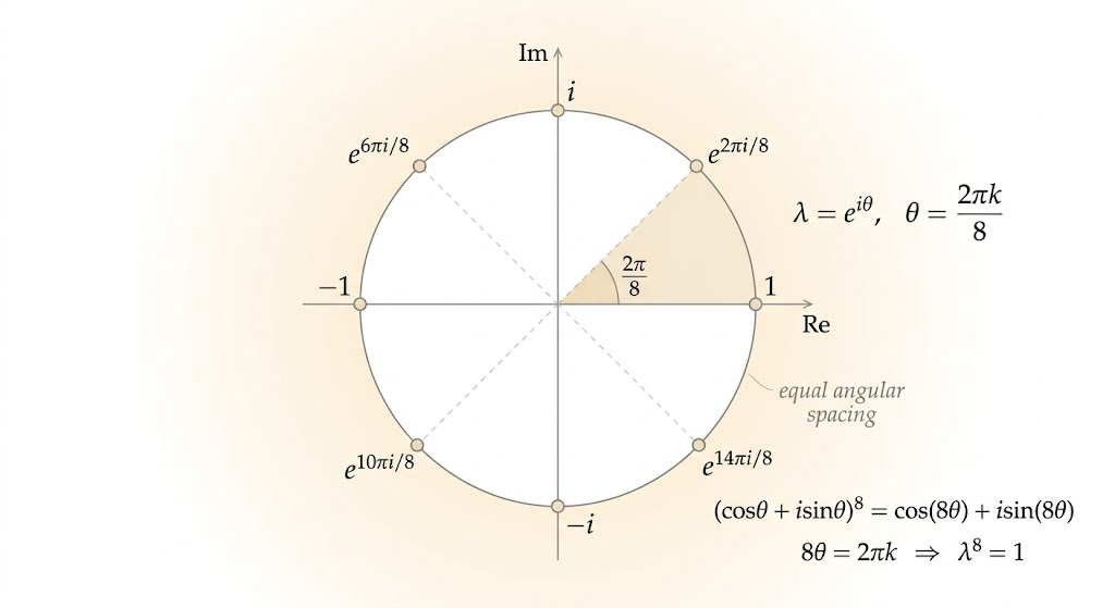
These points lie evenly on the unit circle in the complex plane.
Eigenvectors of P
Now solve the vector equation itself. For the \(4 \times 4\) shift matrix,
\[ Px = \lambda x \]
gives the chain
\[ x_2 = \lambda x_1, \qquad x_3 = \lambda x_2, \qquad x_4 = \lambda x_3, \qquad x_1 = \lambda x_4. \]
If we choose \(x_1 = 1\), then the eigenvector must be
\[ x = \begin{bmatrix} 1 \\ \lambda \\ \lambda^2 \\ \lambda^3 \end{bmatrix}. \]
Substituting the four eigenvalues gives four eigenvectors:
\[ \begin{bmatrix}1\\1\\1\\1\end{bmatrix}, \quad \begin{bmatrix}1\\i\\-1\\-i\end{bmatrix}, \quad \begin{bmatrix}1\\-1\\1\\-1\end{bmatrix}, \quad \begin{bmatrix}1\\-i\\-1\\i\end{bmatrix}. \]
In general, for \(\lambda = \omega^k\), the eigenvector is
\[ v_k = \begin{bmatrix} 1 \\ \omega^k \\ \omega^{2k} \\ \vdots \\ \omega^{(N-1)k} \end{bmatrix}. \]
The Fourier Matrix
Placing these eigenvectors side by side gives the Fourier matrix:
\[ F_N = \begin{bmatrix} 1 & 1 & 1 & \cdots & 1 \\ 1 & \omega & \omega^2 & \cdots & \omega^{N-1} \\ 1 & \omega^2 & \omega^4 & \cdots & \omega^{2(N-1)} \\ \vdots & \vdots & \vdots & \ddots & \vdots \\ 1 & \omega^{N-1} & \omega^{2(N-1)} & \cdots & \omega^{(N-1)^2} \end{bmatrix}. \]
For example, when \(N=8\),
\[ F_8 = \begin{bmatrix} 1 & 1 & 1 & 1 & 1 & 1 & 1 & 1 \\ 1 & W & W^2 & W^3 & W^4 & W^5 & W^6 & W^7 \\ 1 & W^2 & W^4 & W^6 & W^8 & W^{10} & W^{12} & W^{14} \\ 1 & W^3 & W^6 & W^9 & W^{12} & W^{15} & W^{18} & W^{21} \\ 1 & W^4 & W^8 & W^{12} & W^{16} & W^{20} & W^{24} & W^{28} \\ 1 & W^5 & W^{10} & W^{15} & W^{20} & W^{25} & W^{30} & W^{35} \\ 1 & W^6 & W^{12} & W^{18} & W^{24} & W^{30} & W^{36} & W^{42} \\ 1 & W^7 & W^{14} & W^{21} & W^{28} & W^{35} & W^{42} & W^{49} \end{bmatrix}, \]
where \(W = e^{2\pi i/8}\).
Why Fourier Vectors Are Orthogonal
Two different Fourier vectors are orthogonal because their inner product becomes a geometric series:
\[ 1 + \omega^m + \omega^{2m} + \cdots + \omega^{(N-1)m} = 0 \qquad (m \not\equiv 0 \mod N). \]
Geometrically, these terms are equally spaced points on the unit circle, so they cancel out.
After normalization by \(1/\sqrt{N}\), the Fourier matrix becomes unitary:
\[ U_N = \frac{1}{\sqrt{N}} F_N, \qquad U_N^* U_N = I. \]
So the Fourier basis is the orthonormal eigenbasis of the shift matrix.
Orthogonal, Unitary, and Normal Structure
This lecture also sits inside a bigger linear-algebra picture:
- symmetric matrices have real eigenvalues and orthogonal eigenvectors
- diagonal matrices already use the standard basis as eigenvectors
- orthogonal matrices satisfy \(Q^\top Q = I\), so their eigenvalues lie on the unit circle
- skew-symmetric matrices push real vectors into perpendicular directions, which is why their eigenvalues are typically imaginary
- normal matrices are exactly the matrices that can be diagonalized by an orthonormal basis
The Fourier matrix belongs to this picture after normalization: it is unitary, so its columns are orthonormal complex eigenvectors.
Circulant Matrices and Fourier Diagonalization
Since every circulant matrix is a polynomial in \(P\), and \(P\) is diagonalized by the Fourier matrix, every circulant matrix is diagonalized by the same basis:
\[ C = F \Lambda F^{-1}. \]
The eigenvalues of \(C\) are obtained by evaluating the circulant polynomial at the roots of unity.
This is the main structural fact behind fast convolution algorithms.
Connection to Cyclic Convolution
Multiplying a circulant matrix by a vector is the same as cyclic convolution:
\[ Cv = c \circledast v. \]
Because circulant matrices are diagonalized by the Fourier matrix, cyclic convolution can be computed in the Fourier domain:
\[ Cv = F \Lambda F^{-1} v. \]
That is the linear algebra reason the FFT makes convolution fast: convolution becomes diagonal multiplication after moving into the Fourier basis.
Takeaways
- the cyclic shift matrix has eigenvalues equal to the roots of unity
- its eigenvectors are Fourier vectors built from powers of those roots
- the Fourier matrix is the eigenvector matrix of the shift matrix
- every circulant matrix is diagonalized by the same Fourier basis
- cyclic convolution becomes simple multiplication in the Fourier domain