David Silver RL Course - Lecture 5: Model-Free Control
This lecture moves from model-free prediction to model-free control. The goal is no longer just to evaluate a fixed policy. The goal is to improve behavior and eventually learn an optimal policy directly from experience, without knowing the MDP model.
On-Policy Learning
On-policy control means:
- learn about the policy currently being followed
- improve that same policy using the learned value estimates
The usual loop is:
- evaluate the current policy
- improve it
- repeat
In dynamic programming, greedy improvement can be written in terms of the state-value function:
\[ \pi'(s) = \arg\max_a \sum_{s',r} p(s',r \mid s,a)\bigl[r + \gamma v_\pi(s')\bigr]. \]
But this requires the transition model. In model-free control, the useful object is the action-value function:
\[ \pi'(s) = \arg\max_{a \in \mathcal{A}} q_\pi(s,a). \]
So once we estimate \(Q(s,a)\) directly from experience, we can improve the policy without an explicit model.
Greedy and Epsilon-Greedy Improvement
A purely greedy policy chooses the action with the largest estimated action-value:
\[ \pi(s) = \arg\max_a Q(s,a). \]
The problem is exploration. If we always exploit the current estimate, we may stop visiting actions that actually have better long-run value.
The standard fix is an \(\epsilon\)-greedy policy:
- with probability \(1-\epsilon\), choose a greedy action
- with probability \(\epsilon\), choose uniformly at random
If there are \(m\) actions and \(a^*\) is a greedy action, then:
\[ \pi(a \mid s) = \begin{cases} 1-\epsilon+\epsilon/m, & a=a^*, \\ \epsilon/m, & a \neq a^*. \end{cases} \]
This ensures every action keeps a nonzero probability of being tried.
Policy improvement still holds in the \(\epsilon\)-greedy setting: the new \(\epsilon\)-greedy policy with respect to \(q_\pi\) is at least as good as the old one.
GLIE
The lecture emphasizes Greedy in the Limit with Infinite Exploration (GLIE).
The idea is:
- every state-action pair is explored infinitely often
- the policy becomes greedy in the limit
Formally:
\[ \lim_{k\to\infty} N_k(s,a) = \infty \]
for all \((s,a)\), while the exploration rate decays so that the policy becomes nearly greedy. A typical schedule is:
\[ \epsilon_k = \frac{1}{k}. \]
This is the balance control needs:
- enough exploration early
- near-greedy behavior later
Monte Carlo Control
Monte Carlo control uses complete sampled returns to estimate action-values:
\[ q_\pi(s,a) = \mathbb{E}_\pi[G_t \mid S_t=s, A_t=a]. \]
The GLIE Monte Carlo control loop is:
- generate an episode using the current \(\epsilon\)-greedy policy
- for each visited state-action pair, update the action-value estimate from the observed return
- improve the policy to be \(\epsilon\)-greedy with respect to the new \(Q\)
- gradually reduce \(\epsilon\)
Using incremental averaging, the update is
\[ N(S_t,A_t) \leftarrow N(S_t,A_t)+1, \]
\[ Q(S_t,A_t) \leftarrow Q(S_t,A_t) + \frac{1}{N(S_t,A_t)}\bigl(G_t - Q(S_t,A_t)\bigr). \]
This works, but it has the same limitation as Monte Carlo prediction:
- high variance
- must wait for full returns
That leads to TD control.
Sarsa
Sarsa is the on-policy TD control algorithm. Its name comes from the update tuple:
\[ (S_t, A_t, R_{t+1}, S_{t+1}, A_{t+1}). \]
The one-step update is:
\[ Q(S_t,A_t) \leftarrow Q(S_t,A_t) + \alpha\Bigl(R_{t+1} + \gamma Q(S_{t+1},A_{t+1}) - Q(S_t,A_t)\Bigr). \]
This is on-policy because the next action \(A_{t+1}\) is chosen using the same current \(\epsilon\)-greedy policy that the agent is actually following.
So Sarsa evaluates and improves the current behavior policy at the same time.
Under standard conditions:
- GLIE exploration
- Robbins-Monro step sizes
Sarsa converges to the optimal action-value function.
N-Step Sarsa
One-step Sarsa uses only one reward before bootstrapping. Monte Carlo waits until the end. N-step Sarsa sits between them.
Examples:
\[ G_t^{(1)} = R_{t+1} + \gamma Q(S_{t+1},A_{t+1}), \]
\[ G_t^{(2)} = R_{t+1} + \gamma R_{t+2} + \gamma^2 Q(S_{t+2},A_{t+2}), \]
and in general
\[ G_t^{(n)} = R_{t+1} + \gamma R_{t+2} + \cdots + \gamma^{n-1}R_{t+n} + \gamma^n Q(S_{t+n},A_{t+n}). \]
The update becomes
\[ Q(S_t,A_t) \leftarrow Q(S_t,A_t) + \alpha\bigl(G_t^{(n)} - Q(S_t,A_t)\bigr). \]
This is another bias-variance tradeoff:
- small \(n\): more bootstrapping, lower variance
- large \(n\): less bootstrapping, higher variance
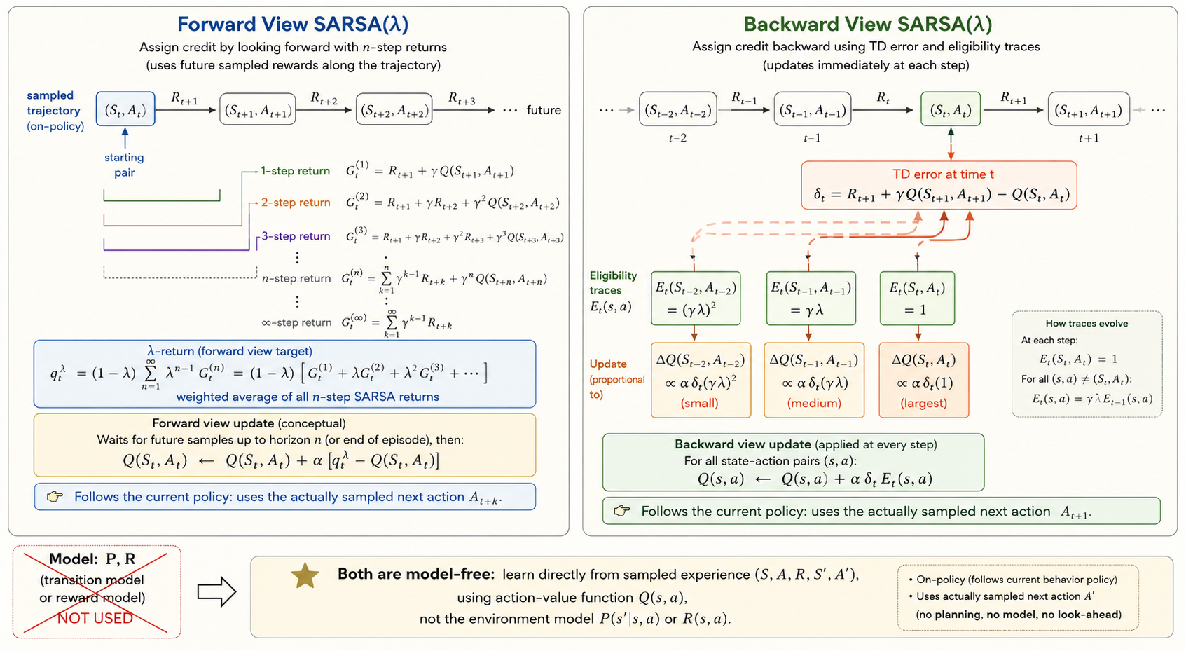
Sarsa(lambda)
Sarsa(\(\lambda\)) combines all n-step returns into one weighted target:
\[ G_t^\lambda = (1-\lambda)\sum_{n=1}^{\infty}\lambda^{n-1} G_t^{(n)}. \]
Then the forward-view update is
\[ Q(S_t,A_t) \leftarrow Q(S_t,A_t) + \alpha\bigl(G_t^\lambda - Q(S_t,A_t)\bigr). \]
The backward view implements the same idea with eligibility traces.
Initialize
\[ E_0(s,a)=0. \]
Then update traces by
\[ E_t(s,a)=\gamma\lambda E_{t-1}(s,a) + \mathbf{1}\{S_t=s,\ A_t=a\}. \]
Define the TD error
\[ \delta_t = R_{t+1} + \gamma Q(S_{t+1},A_{t+1}) - Q(S_t,A_t), \]
and update
\[ Q(s,a) \leftarrow Q(s,a) + \alpha\,\delta_t E_t(s,a). \]
Intuition:
- the most recent actions get the biggest credit or blame
- earlier actions still get updated, but with decayed weight
That is why eligibility traces propagate reward information backward efficiently.
Off-Policy Learning
Off-policy learning separates:
- the behavior policy \(\mu\), which generates data
- the target policy \(\pi\), which we want to evaluate or improve
This matters because it lets us:
- reuse old experience
- learn from exploratory behavior
- learn an optimal greedy policy while still behaving more randomly
Importance Sampling
If samples come from \(\mu\) but we care about expectations under \(\pi\), we correct the mismatch with importance sampling.
Basic identity:
\[ \mathbb{E}_{X\sim P}[f(X)] = \mathbb{E}_{X\sim Q}\left[\frac{P(X)}{Q(X)}f(X)\right]. \]
For off-policy Monte Carlo, we weight returns by the trajectory probability ratio:
\[ \rho_{t:T-1} = \prod_{k=t}^{T-1}\frac{\pi(A_k\mid S_k)}{\mu(A_k\mid S_k)}. \]
Then one ordinary importance-sampling style update is
\[ V(S_t) \leftarrow V(S_t) + \alpha\bigl(\rho_{t:T-1}G_t - V(S_t)\bigr). \]
For one-step TD prediction, only the current-step correction appears:
\[ V(S_t) \leftarrow V(S_t) + \alpha\,\rho_t\Bigl(R_{t+1} + \gamma V(S_{t+1}) - V(S_t)\Bigr), \]
where
\[ \rho_t = \frac{\pi(A_t\mid S_t)}{\mu(A_t\mid S_t)}. \]
Compared with Monte Carlo importance sampling, one-step TD usually has much lower variance.
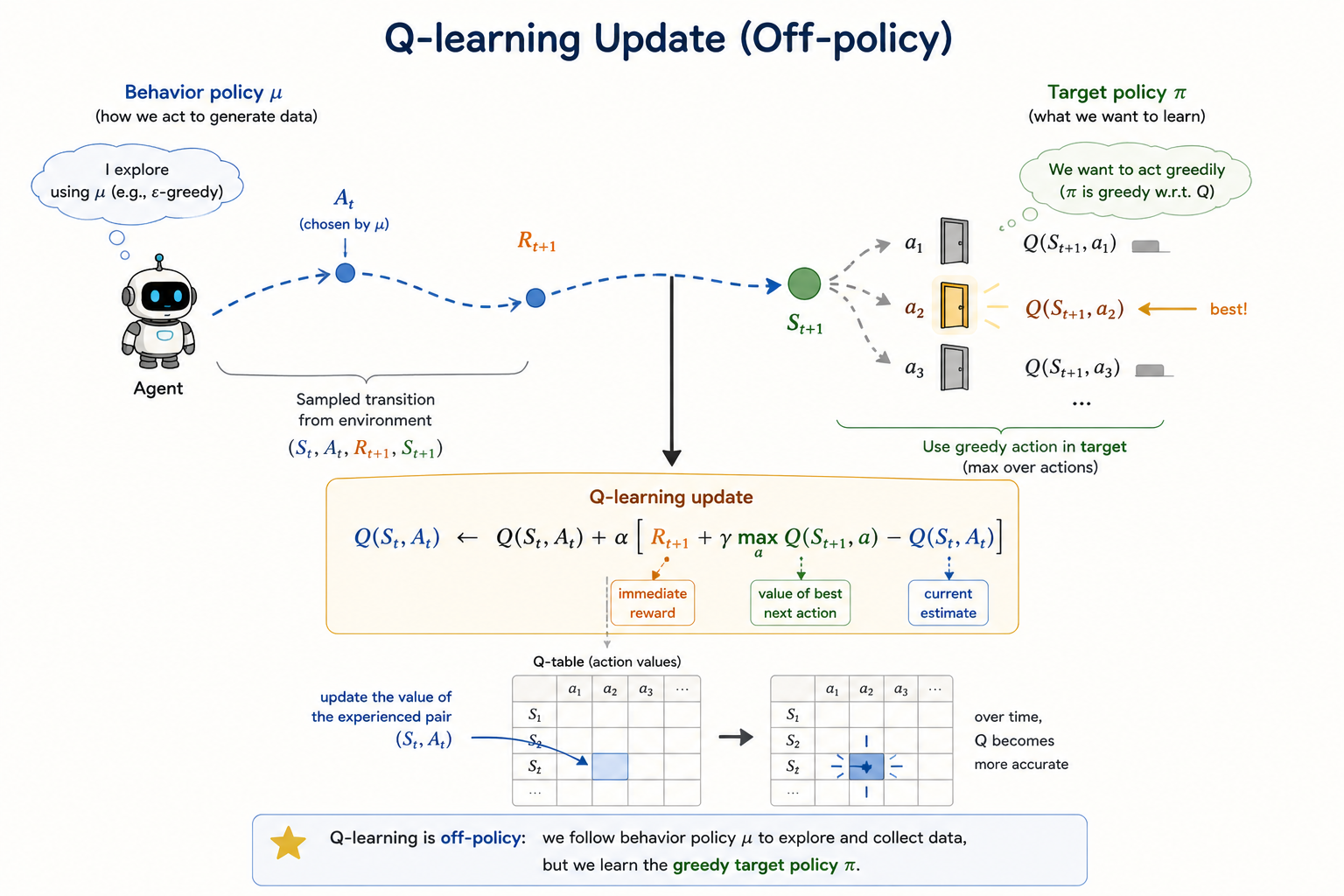
Q-Learning
Q-learning is the key off-policy control method in the lecture.
The update is:
\[ Q(S_t,A_t) \leftarrow Q(S_t,A_t) + \alpha\Bigl(R_{t+1} + \gamma \max_{a'}Q(S_{t+1},a') - Q(S_t,A_t)\Bigr). \]
This is the crucial difference from Sarsa:
- Sarsa bootstraps from the action actually taken next
- Q-learning bootstraps from the best next action according to the current estimate
So Q-learning learns the greedy target policy even while behavior remains exploratory.
That is why no multi-step importance-sampling correction is needed in the control update itself: the target is defined directly by the max operator.
Full Backup vs Sample Backup
This lecture also fits the main RL methods into a useful table:
| Objective | Full Backup (DP) | Sample Backup (TD) |
|---|---|---|
| Bellman expectation for \(v_\pi\) | Iterative policy evaluation | TD learning |
| Bellman expectation for \(q_\pi\) | Policy iteration with action-values | Sarsa |
| Bellman optimality for \(q_*\) | Q-value iteration | Q-learning |
This is a good summary of where model-free control sits:
- dynamic programming uses full expectations from a known model
- TD control uses sampled transitions from experience
Q-Learning Demo
Colab demo:
Summary
- model-free control improves behavior directly from sampled experience
- \(\epsilon\)-greedy policies add exploration to greedy improvement
- GLIE balances infinite exploration with greedy behavior in the limit
- Monte Carlo control learns from complete returns
- Sarsa is the standard on-policy TD control method
- n-step Sarsa and Sarsa(\(\lambda\)) interpolate between one-step bootstrapping and long returns
- off-policy learning separates behavior policy from target policy
- importance sampling corrects policy mismatch
- Q-learning learns the greedy optimal action-value function while behaving exploratorily