Oxford Information Theory Lecture 2: Basic Properties of Information
This lecture is about the structural properties behind the main information-theoretic quantities. The goal is not to define entropy or divergence again, but to understand the inequalities and decomposition rules that make them useful.
Conditional Divergence
Suppose \(p_{Y\mid X}\) and \(q_{Y\mid X}\) are two conditional distributions, and \(p_X\) is the reference distribution over \(X\). The conditional KL divergence is
\[ D\!\left(p_{Y\mid X}\|q_{Y\mid X}\mid p_X\right) = \sum_x p_X(x)\, D\!\left(p_{Y\mid X}(\cdot\mid x)\|q_{Y\mid X}(\cdot\mid x)\right). \]
Equivalently,
\[ D\!\left(p_{Y\mid X}\|q_{Y\mid X}\mid p_X\right) = \mathbb{E}_{X\sim p_X} \left[ D\!\left(p_{Y\mid X}(\cdot\mid X)\|q_{Y\mid X}(\cdot\mid X)\right) \right]. \]
So conditional divergence is just the average mismatch between the two conditional models, weighted by how often each value of \(X\) occurs under the true marginal.
Conditional Mutual Information
For discrete random variables \(X,Y,Z\), the conditional mutual information is
\[ I(X;Y\mid Z)=H(X\mid Z)-H(X\mid Y,Z). \]
Symmetrically,
\[ I(X;Y\mid Z)=H(Y\mid Z)-H(Y\mid X,Z). \]
This measures how much uncertainty about \(X\) is removed by observing \(Y\), once \(Z\) is already known.
Jensen’s Inequality
For a convex function \(\phi\),
\[ \mathbb{E}[\phi(X)] \ge \phi(\mathbb{E}[X]). \]
This inequality is one of the main engines behind information theory. In particular, many non-negativity results come from applying Jensen to the convex function \(-\log x\).
Log-Sum Inequality
Let \(a_1,\dots,a_n\) and \(b_1,\dots,b_n\) be nonnegative numbers. Then
\[ \sum_{i=1}^n a_i \log \frac{a_i}{b_i} \ge \left(\sum_{i=1}^n a_i\right) \log \frac{\sum_{i=1}^n a_i}{\sum_{i=1}^n b_i}. \]
This is the discrete inequality underlying many KL-divergence facts, especially convexity and Gibbs inequality.
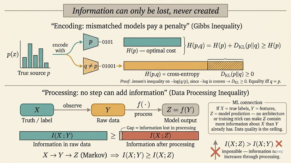
Gibbs Inequality
Let \(p\) and \(q\) be pmfs on the same alphabet. Then
\[ D(p\|q)=\sum_x p(x)\log \frac{p(x)}{q(x)} \ge 0, \]
with equality if and only if \(p=q\).
This can be rewritten as
\[ -\sum_x p(x)\log q(x)\ge -\sum_x p(x)\log p(x). \]
The left-hand side is the cross-entropy \(H(p,q)\), so Gibbs inequality says
\[ H(p,q)\ge H(p). \]
Interpretation: encoding data generated from \(p\) with a mismatched model \(q\) always costs at least as much as using the true distribution itself.
Jensen Proof Sketch
If \(X\sim p\), then
\[ D(p\|q) = \mathbb{E}\left[-\log \frac{q(X)}{p(X)}\right]. \]
Since \(-\log x\) is convex, Jensen gives
\[ \mathbb{E}\left[-\log \frac{q(X)}{p(X)}\right] \ge -\log \mathbb{E}\left[\frac{q(X)}{p(X)}\right] = -\log \sum_x p(x)\frac{q(x)}{p(x)} = -\log 1 =0. \]
Divergence Properties
Let \((X,Y)\) follow the true joint distribution \(P_{XY}\), and let \((\hat X,\hat Y)\) denote a model joint distribution \(P_{\hat X\hat Y}\) on the same space.
1. Information Inequality
For any two pmfs,
\[ D(P_X\|P_{\hat X})\ge 0. \]
This is just Gibbs inequality applied to the marginals.
2. Chain Rule for Divergence
The divergence between joint distributions decomposes as
\[ D(P_{XY}\|P_{\hat X\hat Y}) = D(P_X\|P_{\hat X}) + D(P_{Y\mid X}\|P_{\hat Y\mid \hat X}\mid P_X). \]
This is one of the most useful structural formulas in information theory: mismatch in the joint law equals mismatch in the marginal plus mismatch in the conditional.
3. Monotonicity Under Marginalization
Because conditional divergence is nonnegative,
\[ D(P_{XY}\|P_{\hat X\hat Y})\ge D(P_X\|P_{\hat X}). \]
Looking at the full joint distribution can only reveal more mismatch than looking at the marginal alone.
4. Equivalent Form of Conditional Divergence
Conditional divergence can be rewritten as an ordinary KL divergence:
\[ D(P_{Y\mid X}\|P_{\hat Y\mid \hat X}\mid P_X) = D(P_XP_{Y\mid X}\|P_XP_{\hat Y\mid \hat X}). \]
This says: if both models use the same true marginal over \(X\), then the remaining divergence is exactly the cost of getting the conditional distribution of \(Y\) wrong.
5. Joint Convexity
For \(\lambda\in[0,1]\),
\[ D(\lambda p_1+(1-\lambda)p_2\|\lambda q_1+(1-\lambda)q_2) \le \lambda D(p_1\|q_1)+(1-\lambda)D(p_2\|q_2). \]
So KL divergence is jointly convex in both arguments. Mixtures do not increase divergence beyond the corresponding weighted average.
Mutual Information Properties
1. Nonnegativity
\[ I(X;Y)\ge 0, \]
with equality if and only if \(X\) and \(Y\) are independent.
Since
\[ I(X;Y)=D(P_{XY}\|P_XP_Y), \]
this is another direct consequence of KL nonnegativity.
2. Symmetry and Entropy Reduction
\[ I(X;Y)=I(Y;X)=H(X)-H(X\mid Y)=H(Y)-H(Y\mid X). \]
So mutual information is exactly the reduction in uncertainty produced by observation of the other variable.
3. Chain Rule for Mutual Information
For a sequence \(X_1,\dots,X_n\),
\[ I(X_1,\dots,X_n;Y) = \sum_{i=1}^n I(X_i;Y\mid X_1,\dots,X_{i-1}). \]
This expresses total information as a step-by-step accumulation of new information revealed by each variable.
4. Data Processing Inequality
If \(X\to Y\to Z\) forms a Markov chain, meaning \(X\perp Z\mid Y\), then
\[ I(X;Y)\ge I(X;Z). \]
Post-processing cannot create new information about the original source.
5. Deterministic Processing
If \(Z=f(Y)\) for a deterministic function \(f\), then
\[ I(X;Y)\ge I(X;f(Y)). \]
This is a special case of the data processing inequality.
Entropy Properties
1. Bounds on Entropy
If \(X\) takes values in a finite alphabet \(\mathcal X\), then
\[ 0\le H(X)\le \log |\mathcal X|. \]
The lower bound is achieved when \(X\) is deterministic; the upper bound is achieved when \(X\) is uniform.
2. Conditioning Reduces Entropy
\[ 0\le H(X\mid Y)\le H(X). \]
Equality cases:
- \(H(X\mid Y)=H(X)\) iff \(X\) and \(Y\) are independent
- \(H(X\mid Y)=0\) iff \(X\) is a deterministic function of \(Y\)
3. Chain Rule and Subadditivity
\[ H(X_1,\dots,X_n) = \sum_{i=1}^n H(X_i\mid X_1,\dots,X_{i-1}) \le \sum_{i=1}^n H(X_i). \]
The inequality becomes equality exactly when the variables are independent.
4. Entropy of a Function
For any deterministic function \(f\),
\[ H(f(X))\le H(X), \]
with equality if \(f\) is injective on the support of \(X\).
A function can merge outcomes and lose information, but it cannot create extra uncertainty beyond what was already present in \(X\).
5. i.i.d. Sequences
If \(X_1,\dots,X_n\) are i.i.d., then
\[ H(X_1,\dots,X_n)=nH(X_1). \]
There is no overlap to subtract because independence makes the joint entropy additive.
Machine Learning Connection
Two points matter immediately for machine learning:
- data processing says post-processing features cannot magically create information about the target that was not already present
- KL-based objectives and entropy inequalities explain why likelihood, cross-entropy, compression, and distribution matching are all tightly connected
This lecture is useful because it turns information theory from a list of formulas into a small set of structural laws: nonnegativity, chain rules, convexity, and monotonicity under processing.